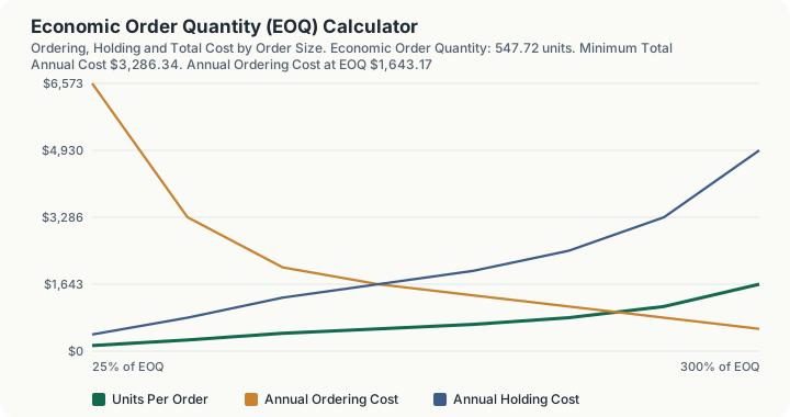
Quick Answer: With annual demand of 12,000 units, $75 to place an order and $6 a year to hold one unit, the economic order quantity is 547.72 units: 21.91 orders a year, roughly one every 16.7 days, at a total annual cost of $3,286.34 split evenly between ordering and holding. Ordering 20% more costs only 1.67% extra a year, so the curve is nearly flat.
What does this calculator do?
The economic order quantity is the oldest result in inventory theory, published by Ford Harris in 1913, and it answers exactly one question: given a steady rate of consumption, how much should you buy at a time? Two costs pull in opposite directions. Ordering frequently means many fixed order costs a year but very little stock sitting on a shelf. Ordering rarely means few order costs but a warehouse full of capital. EOQ is the order size at which those two costs are balanced.
The result has a striking property that matters more commercially than the formula itself: at the optimum, annual ordering cost and annual holding cost are exactly equal. That is not a coincidence, it is what setting the derivative to zero produces, and it gives you a free sanity check on any EOQ you compute. If the two figures do not match, something is wrong.
The second property that matters is flatness. The total cost curve near its minimum is very nearly horizontal. Ordering 20% above EOQ costs 1.67% more; even doubling the order size costs only 25% more. This has a blunt practical consequence: precision in the inputs is worth much less than people assume. If your supplier ships in cases of 500, order 500 rather than 547.72 and you lose almost nothing. The model's assumptions (constant known demand, instant replenishment, no quantity discounts, no capacity limit) fail long before the arithmetic does.
How is this calculated?
Annual cost of an order quantity $Q$, given annual demand $D$, order cost $S$ and holding cost $H$ per unit per year:
TC(Q) = D/QS + Q/2H
Setting the derivative to zero gives
Q^∗ = √(2DS/H); TC(Q^∗) = √2DSH
Step 1: Build the numerator. 2 x 12,000 x $75 = 1,800,000
Step 2: Divide by the holding cost. 1,800,000 / 6 = 300,000
Step 3: Take the square root. sqrt(300,000) = 547.72 units
Step 4: Compute orders per year. 12,000 / 547.72 = 21.91 orders
Step 5: Compute the interval between orders. 365 / 21.91 = 16.7 days
Step 6: Compute the annual ordering cost at the optimum. 21.91 x $75 = $1,643.17
Step 7: Compute the annual holding cost at the optimum. Average inventory is half the order quantity: 547.72 / 2 = 273.86 units. 273.86 x $6 = $1,643.17
These two are equal, and that equality is the definition of the optimum.
Step 8: Total annual cost. $1,643.17 + $1,643.17 = $3,286.34
This equals sqrt(2 x 12,000 x 75 x 6) = sqrt(10,800,000) = $3,286.34, as the closed form predicts.
Step 9: Compute the reorder point. Daily demand: 12,000 / 365 = 32.88 units. 32.88 x 14 days of lead time = 460.27 units
The reorder point answers when to order, not how much. It is independent of the EOQ.
Step 10: Measure the flatness of the curve. Because TC(kQ^∗)/TC(Q^∗) = (1/k + k)/2: at k = 1.2: (1/1.2 + 1.2)/2 = 1.67% above optimal at k = 0.8: (1/0.8 + 0.8)/2 = 2.50% above optimal
Worked Example
A distributor sells 12,000 units a year. Each purchase order costs $75 in paperwork, freight minimum and inspection regardless of size. Holding one unit for a year costs $6 in storage, insurance, shrinkage and tied-up capital. The supplier takes 14 days.
Step 1: Test ordering monthly, 1,000 units at a time. Ordering cost: 12 x $75 = $900.00 Holding cost: 500 average units x $6 = $3,000.00 Total: $3,900.00
Step 2: Test ordering weekly, about 231 units at a time. Ordering cost: 12,000 / 231 x $75 = $3,896.10 Holding cost: 115.5 x $6 = $693.00 Total: $4,589.10
Step 3: Compute the optimum instead. sqrt(2 x 12,000 x 75 / 6) = 547.72 units
Step 4: Total cost at the optimum. $1,643.17 + $1,643.17 = $3,286.34
Step 5: The saving against monthly ordering. $3,900.00 - $3,286.34 = $613.66 a year, about 15.7%.
Step 6: The saving against weekly ordering. $4,589.10 - $3,286.34 = $1,302.76 a year, about 28.4%.
Step 7: Now round to a convenient case size of 550. Ordering: 12,000 / 550 x $75 = $1,636.36 Holding: 275 x $6 = $1,650.00 Total: $3,286.36, two cents worse than the exact optimum. Round freely.
Step 8: Set the reorder point. Place the next order when stock falls to 460.27 units, so the delivery arrives as the shelf empties.
Note how weakly EOQ responds to its inputs. Quadrupling the order cost to $300 only doubles the EOQ to 1,095.45 units, because the square root damps everything. Doubling the holding cost to $12 shrinks EOQ to 387.30 units, a fall of only 29%. Tripling demand to 36,000 raises EOQ to 948.68 units, well under triple, which is why order frequency has to rise as a business grows.
What does this calculator not account for?
- Quantity discounts. The model assumes unit price is constant. Where a supplier offers a lower price at a higher volume, the correct method compares total cost including purchase price at each price break, and the answer is frequently a break quantity rather than the EOQ.
- Safety stock and demand variability. The reorder point here is purely deterministic: daily demand multiplied by lead time. It carries no buffer for demand spikes or late deliveries, and any real operation needs one.
- Lead time variability. Lead time is treated as a fixed number of days.
- Seasonality and trend. Demand is assumed steady and known for the whole year. A product with a Christmas peak is badly served by a single annual EOQ.
- Storage and cash constraints. Nothing here checks whether you have room for 547.72 units or the working capital to buy them.
- Perishability and obsolescence, beyond whatever you fold into the holding cost figure.
- Multiple products competing for the same budget, space or delivery slots. The formula optimises one item in isolation.
- Backorders and stockout costs. The model assumes replenishment is instantaneous at the reorder point and demand is never lost.
- The 365-day year. Daily demand is annual demand divided by 365 calendar days, not working days, which will understate daily demand for an operation that ships five days a week.
What mistakes do people make with this?
- Chasing precision in the inputs. The cost curve is flat: a 20% error in the order quantity costs under 2%. Time spent refining a holding cost estimate from $6 to $6.30 is time wasted, and the assumptions behind the model are a far larger source of error than the arithmetic.
- Forgetting that holding cost is annual and per unit. A common error is entering the cost of holding the whole order, or a monthly figure. Both wreck the answer, and the wrongness is not obvious because the square root hides it.
- Omitting the cost of capital from holding cost. Storage and insurance are visible; the money tied up in stock is not, and for expensive items it is usually the largest component.
- Treating the reorder point as an order quantity. They are separate answers to separate questions. On the defaults the reorder point of 460.27 units is close to the EOQ of 547.72, which invites confusion, but the two are unrelated quantities.
- Applying EOQ where demand is lumpy. For an item ordered three times a year against specific projects, the formula's constant-demand assumption is simply false and the answer is meaningless.
- Ignoring supplier minimums and case sizes. If the supplier ships in pallets of 400, your real choice is 400 or 800, and the flatness of the curve tells you which is cheaper without any further theory.
- Assuming the two cost lines should not be equal. If your ordering and holding costs at the computed EOQ differ, you have made an arithmetic error somewhere.
Frequently Asked Questions
Why are ordering cost and holding cost exactly equal at the EOQ?
How much does it cost me to get the order quantity wrong?
Does EOQ tell me when to reorder?
What should I include in the holding cost per unit?
Why doesn't tripling my demand triple the order size?
Sources
- U.S. Small Business Administration, the official authority for the business this calculator relates to. sba.gov
Also consulted: Ford W. Harris, "How Many Parts to Make at Once", Factory: The Magazine of Management, volume 10, number 2 (1913), pages 135-136 and 152. The original derivation of the square-root order quantity. It remains the model implemented here; The total cost function TC(Q) = D/QS + Q/2H, its minimiser Q^∗ = √(2DS/H), the minimum cost √2DSH, and the sensitivity ratio $(1/k+k)/2$ are all elementary consequences of that function and are what this engine computes.
No authority publishes EOQ parameters, and no primary source is cited for any input, because none exists. Order costs and holding costs are properties of your own operation, and no government, regulatory or standards body publishes normal ranges for them. The defaults here (12,000 units of annual demand, $75 per order, $6 per unit per year, 14 days of lead time) are illustrative values chosen to demonstrate the arithmetic, not benchmarks. The mathematics is a standard published result: