Risk Parity Calculator (Equal Risk Contribution)

Sleeve	Capital Weight %	Risk Share %	Risk Less Capital (pp)
Equities (comparison)	$60.00	$91.21	$31.21
Bonds (comparison)	$40.00	$8.79	$-31.21
Equities (risk parity)	$27.27	$50.00	$22.73
Bonds (risk parity)	$72.73	$50.00	$-22.73

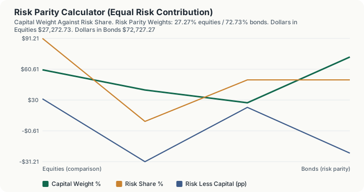
Quick Answer: At the defaults -- 16% equity volatility, 6% bond volatility and a 0.15 correlation -- a conventional 60/40 portfolio puts 60% of the capital in equities and gets 91.21% of its risk from them. Weighting by the inverse of volatility gives 27.27% equities and 72.73% bonds, which is the mix where each sleeve contributes exactly half the portfolio risk. Volatility falls from 10.24% to 6.62%.

Overview

A 60/40 portfolio is not a balanced portfolio. It is balanced by capital and wildly unbalanced by risk, because equities are roughly three times as volatile as bonds and risk contribution scales with volatility rather than with dollars. At the default assumptions, the 40% bond sleeve supplies under 9% of the portfolio's variability. Whatever the investor believes they own, what they own is an equity portfolio with a small cash-like hedge.

Risk parity starts from the opposite constraint. Rather than choosing the capital weights and accepting whatever risk split falls out, it chooses the weights so each sleeve contributes the same share of risk. For two assets, the solution is simply the inverse of the volatilities: hold less of what moves more, in exact proportion.

This calculator computes both mixes side by side, reports how much risk each sleeve actually supplies in each, and converts the risk-parity weights into dollars. The comparison mix is yours to set, so 60/40 is only the default, not a fixed reference.

How This Is Calculated

Risk contributions come from the standard decomposition of portfolio variance. For asset $i$ with weight $w_i$:

\text{risk share}_i = \frac{w_i (\Sigma w)_i}{\sigma_p^2}, \qquad (\Sigma w)_i = \sum_j w_j \sigma_{ij}

The covariance matrix is built from the volatilities and one uniform pairwise correlation applied to every off-diagonal pair. There is no correlation matrix to fill in and none is estimated: a single number describes the relationship between every pair of sleeves. Diagonal entries are the variances.

Step 1 -- Compute the inverse-volatility weights. 1 / 16 = 0.0625 1 / 6 = 0.166667 Sum: 0.229167

Step 2 -- Normalise them. 0.0625 / 0.229167 = 0.272727 = 27.27% equities 0.166667 / 0.229167 = 0.727273 = 72.73% bonds

Step 3 -- Convert to dollars on a $100,000 portfolio. $100,000 x 0.272727 = $27,272.73 in equities $100,000 x 0.727273 = $72,727.27 in bonds

Step 4 -- Compute the covariance between the two sleeves. 0.15 x 0.16 x 0.06 = 0.00144

Step 5 -- Compute the comparison portfolio's variance at 60/40. 0.60² x 0.16² = 0.009216 0.40² x 0.06² = 0.000576 2 x 0.60 x 0.40 x 0.00144 = 0.0006912 Total: 0.0104832

Step 6 -- Take its volatility. $\sqrt{0.0104832}$ = 10.24%

Step 7 -- Compute the equity risk contribution in that comparison mix. $(\Sigma w)_{eq}$ = (0.60 x 0.0256) + (0.40 x 0.00144) = 0.01536 + 0.000576 = 0.015936 Risk contribution: 0.60 x 0.015936 = 0.0095616 Risk share: 0.0095616 / 0.0104832 = 91.21%

Step 8 -- Measure how far risk runs ahead of capital. 91.21% - 60.00% = 31.21 percentage points

Step 9 -- Compute the risk-parity portfolio's variance. 0.272727² x 0.0256 = 0.0019040 0.727273² x 0.0036 = 0.0019041 2 x 0.272727 x 0.727273 x 0.00144 = 0.0005711 Total: 0.0043791

The first two terms being equal to four decimal places is the equal-risk property showing up directly in the arithmetic.

Step 10 -- Take its volatility. $\sqrt{0.0043791}$ = 6.62%

Step 11 -- Confirm the risk split. 50.00% each. For two assets, inverse-volatility weighting equalises risk contributions exactly, and it does so at any shared correlation level, because the correlation term enters both contributions symmetrically. This is why changing the correlation input moves portfolio volatility but leaves the risk-parity weights untouched.

Step 12 -- Measure the volatility given up. 10.24% - 6.62% = 3.62 percentage points

Worked Example

You hold $100,000 in a conventional 60/40 split and want to know what you actually own.

Step 1 -- The capital split you chose. $60,000 equities, $40,000 bonds.

Step 2 -- The risk split you got. 91.21% equities, 8.79% bonds.

The bond sleeve is 40% of the money and under a tenth of the risk. In practice this portfolio does what equities do, slightly damped. Its drawdowns, its correlations to other holdings, and its behaviour in a crisis are equity behaviour.

Step 3 -- The gap between the two. 31.21 percentage points of risk sitting ahead of capital.

Step 4 -- What equal risk contribution requires. 27.27% equities, 72.73% bonds, or $27,272.73 and $72,727.27.

Step 5 -- The resulting risk split. 50.00% each. Exactly balanced, by construction.

Step 6 -- The cost. Portfolio volatility drops from 10.24% to 6.62%, a reduction of 3.62 points. That is not free. A calmer portfolio holding far more of the lower-returning asset should be expected to return less. This calculator computes no returns and applies no leverage, so it shows only half of the trade.

Step 7 -- Test how robust the weights are. Change the correlation from 0.15 to 0.80. Portfolio volatility rises for both mixes, but the risk-parity weights stay at exactly 27.27% / 72.73%, because for two assets they depend only on the ratio of the volatilities. Change the bond volatility to 3% instead and the weights move sharply, to 15.79% equities. The volatility estimate is the assumption that matters here; the correlation is not.

What This Does Not Account For

Leverage, which is how risk parity is actually run. The strategy in practice borrows to lever the low-volatility sleeve back up to a target risk level, so the portfolio is not simply a calmer, lower-returning version of 60/40. Nothing here models borrowing, financing cost, margin, or the leverage-induced tail risk that follows. The unlevered comparison shown is only the first half of the idea.
A full covariance matrix. All pairs share a single correlation figure. That is a real simplification, stated explicitly rather than hidden, and it is why this page handles two sleeves rather than nine.
Expected returns. None are used and none are produced. Risk parity is a risk-allocation rule and this page implements only the risk half. Whether the resulting portfolio has an adequate expected return is not addressed.
Volatility estimation. The 16% and 6% defaults are illustrative round numbers near long-run figures for broad equity and investment-grade bond indices. They are not sourced, and the weights are entirely determined by them.
Time-varying risk. Volatilities and correlations are fixed inputs. Real risk-parity implementations re-estimate them continuously and rebalance, which introduces turnover, cost, and the possibility of raising leverage into a volatility spike.
Rebalancing, transaction costs and taxes. The weights are treated as static.
Non-normal returns. Volatility weights gains and losses equally and says nothing about drawdown shape, skew or tails. A bond sleeve that is calm for years and then is not will look safe here right up until it does not.
Inflation and duration risk in the bond sleeve. Holding 72.73% in bonds concentrates a different exposure that volatility alone does not describe.

Common Pitfalls

Believing 60/40 is diversified. The 91.21% figure is the whole point of this page. Capital balance and risk balance are different things, and the difference is large.
Expecting risk parity to beat 60/40 unlevered. It should not, and this calculator shows why: it is a substantially calmer portfolio, which ordinarily means a lower-returning one. The case for risk parity depends on levering the calmer portfolio back to a comparable risk level, which is outside this model.
Assuming the weights depend on correlation. For two assets they do not. Only the volatility ratio matters. The correlation changes the resulting portfolio volatility, not the mix.
Using stale volatility estimates. The weights are a direct function of the volatility ratio. A bond volatility estimate taken from a low-rate decade produces a very different allocation than one taken from a rate-shock year.
Reading equal risk contribution as equal risk of loss. Both sleeves supply half the variance. That is a statement about co-movement, not a promise that losses arrive in equal size or at the same time.
Applying two-asset intuition to many assets. Inverse-volatility weighting equalises risk contributions exactly for two sleeves under a shared correlation. With many assets and a genuine correlation matrix it is an approximation, and the true equal-risk-contribution solution requires numerical optimisation.

Frequently Asked Questions

Why does a 60/40 portfolio get 91% of its risk from stocks?

Because risk contribution scales with volatility, not with dollars. Equities at 16% volatility are roughly 2.7 times as variable as bonds at 6%, and variance scales with the square, so the equity sleeve dominates the total even at a modest capital weight. The 40 cents in bonds absorbs 8.79% of the variability. That is the observation the entire risk parity literature is built on.

Do the risk parity weights change if correlation changes?

For a two-asset portfolio, no. Set the correlation to 0.80 or to -0.20 and the weights stay at 27.27% / 72.73%, because the correlation term contributes symmetrically to both risk contributions and cancels out of the equalisation. What does change is the portfolio's volatility. The engine confirms this: it reports the mix as risk balanced across the whole correlation range.

Is risk parity just a bond-heavy portfolio?

Unlevered, yes, and that is a fair criticism of the version shown here. The strategy as practised applies leverage to the low-volatility sleeve to raise expected return back to a comparable level. That leverage carries financing cost and its own failure mode, and it is not modelled on this page. Read the 27.27% / 72.73% mix as the risk-balanced starting point, not as a complete strategy.

Why does volatility fall by so much less than the equity weight does?

Equity weight falls from 60% to 27.27%, a cut of more than half, while volatility falls only from 10.24% to 6.62%, about 35%. Diversification is already doing some of the work at 60/40, and the bond sleeve carries volatility of its own. Risk reduction is a square-root function of the weights, so it flattens out.

What volatility figures should I use?

Annualised standard deviations measured over a period relevant to your horizon, both at the same frequency. The weights are wholly determined by the ratio between them, so the two estimates must be consistent with each other above all else. Note that the defaults here are illustrative and are not a quote from any index.

Does this work for more than two sleeves?

The primitive is written for a list of assets and a shared correlation, so the risk decomposition generalises. This calculator exposes two sleeves. Beyond two assets, inverse-volatility weighting no longer equalises risk contributions exactly unless the correlations really are all identical, so treat it as an approximation.

Sources

The risk contribution decomposition $RC_i = w_i(\Sigma w)_i / \sigma_p^2$ is the standard Euler allocation of portfolio variance; the engine implements it directly and normalises the supplied weights before use.
Maillard, S., Roncalli, T., and Teiletche, J., "The Properties of Equally Weighted Risk Contribution Portfolios," Journal of Portfolio Management, 2010. The formal treatment of equal risk contribution and of the inverse-volatility solution.
Qian, E., "Risk Parity Portfolios: Efficient Portfolios Through True Diversification," 2005.
The covariance matrix used here is constructed from the supplied volatilities and a single uniform pairwise correlation, not from an estimated correlation matrix.

Risk Parity Calculator (Equal Risk Contribution)

Assumptions

Preset scenarios

Capital Weight Against Risk Share