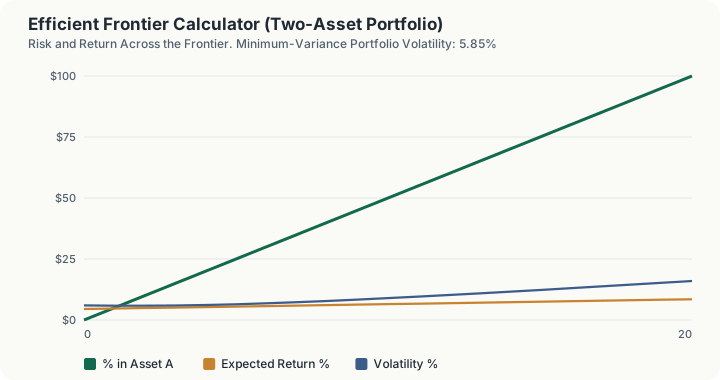
Quick Answer: Pairing an asset returning 8.5% at 16% volatility with one returning 4.5% at 6% volatility, at a correlation of 0.15, the minimum-variance portfolio is 8.21% in the first and 91.79% in the second, with a volatility of 5.85% and an expected return of 4.83%, less volatile than either asset alone. Among the 21 weights sampled, the highest Sharpe mix is 70% / 30%.
What does this calculator do?
Combining two assets does something that combining two of anything else does not: the risk of the combination can be lower than the risk of either component. Returns blend linearly: a 70/30 mix earns 70% of one return plus 30% of the other, always. Risk does not, and the whole of modern portfolio theory lives in that gap.
The reason is that variance depends on how the two assets move together, not just on how much each moves. When one asset is down and the other is flat or up, the losses partly cancel, and the more independently they move the more cancellation there is. Correlation is the parameter that governs it, and it is the only input on this page that bends the curve. At a correlation of exactly 1 the assets are redundant, the frontier straightens into a line, and no mix beats a weighted average of the two.
This calculator traces the frontier across 21 weightings from 0% to 100% in one asset, and identifies three points on it: the minimum-variance portfolio, the equal-weighted mix for reference, and the highest-Sharpe mix among the weights sampled. It also tells you whether the minimum-variance mix beats both standalone assets on volatility, which is the sharpest statement diversification makes.
Only the arc above the minimum-variance point is efficient. Below it, every portfolio is dominated: there is another mix with the same volatility and a higher expected return. That is why the minimum-variance point matters far beyond being the calmest option.
How is this calculated?
σₚ² = w_A²σ_A² + w_B²σ_B² + 2w_Aw_Bρσ_Aσ_B
E(Rₚ) = w_AR_A + (1 − w_A)R_B; Sharpe = (E(Rₚ) − R_f)/σₚ
w_A^∗ = (σ_B² − ρσ_Aσ_B)/(σ_A² + σ_B² − 2ρσ_Aσ_B)
Step 1: Convert the percentage volatilities into decimals. Each volatility input is divided by 100 before any variance arithmetic.
Step 2: Compute the covariance. Correlation multiplied by both volatilities. This single number carries the whole interaction between the two assets.
Step 3: Solve for the minimum-variance weight in closed form. Asset B's variance less the covariance, divided by the sum of both variances less twice the covariance. The result is clamped into the range 0 to 1, so the calculator never reports a short position. When the denominator is exactly zero it falls back to a 50/50 split.
Step 4: Compute the volatility at that weight. The two-asset variance formula is applied to the minimum-variance weights, and the square root taken.
Step 5: Compute the return at that weight. The weighted average of the two expected returns. Return is always linear in the weight, whatever the correlation is.
Step 6: Sweep the frontier. The same two calculations are repeated for 21 weights running from 0% to 100% in the first asset, in 5-point steps.
Step 7: Compute a Sharpe ratio at each sampled weight. Expected return less the risk-free rate, divided by that mix's volatility. The risk-free rate enters the calculation here and nowhere else.
Step 8: Pick the highest-Sharpe point among those sampled. The calculator scans the 21 sampled weights and reports the best. This is a grid search over the sampled weights, not an analytic solution for the tangency portfolio, so the reported mix will always land on a 5-point increment.
Step 9: Compute the equal-weighted volatility. The same variance formula at a 50/50 split, reported for reference.
Step 10: Test whether the minimum-variance mix beats both assets. Its volatility is compared against the lower of the two standalone volatilities, and the reading is set accordingly.
Each frontier point also carries an efficiency flag: points below the minimum-variance weight, on the side away from the higher-returning asset, are marked as dominated.
Worked Example
Defaults: asset A returns 8.5% with 16% volatility, asset B returns 4.5% with 6% volatility, correlation 0.15, risk-free rate 4%.
Step 1: Compute the covariance. 0.15 × 0.16 × 0.06 = 0.00144
Step 2: Compute the minimum-variance numerator. 0.06² − 0.00144 = 0.0036 − 0.00144 = 0.00216
Step 3: Compute the denominator. 0.16² + 0.06² − (2 × 0.00144) = 0.0256 + 0.0036 − 0.00288 = 0.02632
Step 4: Solve for the minimum-variance weight. 0.00216 ÷ 0.02632 = 0.08207, so 8.21% in asset A and 91.79% in asset B
Step 5: Compute the variance at that mix. (0.08207² × 0.0256) + (0.91793² × 0.0036) + (2 × 0.08207 × 0.91793 × 0.00144) = 0.00017243 + 0.00303305 + 0.00021698 = 0.00342246
Step 6: Take the square root. √0.00342246 = 0.05850, or 5.85% volatility
Step 7: Note that this beats both assets alone. 5.85% is below asset B's own 6.00%, so a small allocation to the riskier asset lowered total risk
Step 8: Compute the return at the minimum-variance mix. (0.08207 × 8.5%) + (0.91793 × 4.5%) = 0.70% + 4.13% = 4.83%
Step 9: Compute the 50/50 mix for contrast. Variance = (0.25 × 0.0256) + (0.25 × 0.0036) + (2 × 0.25 × 0.00144) = 0.00802, so volatility = 8.96%, well below the 11.00% simple average of 16% and 6%
Step 10: Find the best Sharpe among the sampled weights. At 70% A / 30% B: return = 7.30%, volatility = 11.61%, and (7.30% − 4.00%) ÷ 11.61% = 0.284
Step 7 is the result worth pausing on. Adding 8.21% of a 16%-volatility asset to a 6%-volatility asset made the portfolio calmer than the calm asset alone. Nothing about the individual assets changed; only their low correlation made it possible.
What does this calculator not account for?
- Exactly two assets. This is the two-asset case, with one correlation. It does not build a covariance matrix, does not accept three or more assets, and cannot express the correlation structure of a real multi-asset portfolio.
- No short selling and no leverage. The minimum-variance weight is clamped to the 0-to-100% range, and the frontier sweep runs only over long-only weights. Portfolios that short one asset to buy more of the other are outside the model.
- The tangency portfolio is sampled, not solved. The highest-Sharpe mix is the best of 21 weights on a 5-point grid. The true tangency portfolio generally lies between grid points, so the reported Sharpe is a floor on the achievable one.
- No capital market line. The risk-free rate is used only to rank mixes by Sharpe. The calculator does not build combinations of the risk-free asset with the tangency portfolio.
- Expected returns, volatilities and correlation are inputs with no authority. Nothing on this page is sourced from a data provider. Optimisers are notoriously sensitive to expected return estimates, and a small change in an input you guessed at can move the optimal mix substantially.
- Correlation is treated as stable. It is not. Correlations between risky assets typically rise sharply in market stress, which removes diversification exactly when it is needed. The calculator will show you that regime if you enter it, but it will not predict it.
- Volatility as the only risk measure. Standard deviation treats upside and downside symmetrically and says nothing about skew, fat tails or drawdown depth.
- Single period, no rebalancing, no costs and no taxes. There is no multi-period compounding, no rebalancing drag or benefit, and no transaction cost on reaching the target weights.
- The square root is taken in floating point, so volatility figures carry ordinary double precision rather than exact decimal arithmetic.
What mistakes do people make with this?
Confusing the minimum-variance portfolio with the best portfolio. It is the calmest, not the best. It sits at the far left of the curve, and every point above it on the arc offers more return for more risk. Which of those you want depends on your risk tolerance, not on the mathematics.
Holding a portfolio below the minimum-variance point. Any mix with less of the higher-returning asset than the minimum-variance weight is dominated: there is another mix with identical volatility and higher expected return. Those points are on the curve but they are never rational to hold.
Assuming correlation is a fixed property. At 0.15 the minimum-variance mix here is calmer than either asset. Push correlation to 0.8 and most of that benefit vanishes. Crisis correlations are typically far higher than long-run averages, which is why backtested diversification often disappoints in the events it was meant to survive.
Treating a correlation of 1 as a special case worth avoiding. It is worth understanding: at a correlation of exactly 1 the frontier collapses into a straight line, the minimum-variance mix becomes 100% of the calmer asset, and no combination beats a weighted average. That is the baseline against which every diversification claim should be read.
Over-trusting an optimiser fed with guessed returns. The weights are extremely sensitive to expected returns. Nudging one return input by a point can move the highest-Sharpe mix by tens of percentage points, which is why practitioners often anchor on the minimum-variance portfolio, since it does not use expected returns at all.
Forgetting that negative correlation goes further. At −0.3 the curve bends further left and the minimum-variance mix is calmer still. Genuinely negatively correlated pairs are rare and their correlations are unstable.
Frequently Asked Questions
What is the efficient frontier?
How can a portfolio be less volatile than both of its components?
What is the minimum-variance portfolio and why does it matter?
What does the correlation input actually change?
Is the tangency portfolio the same as the highest-Sharpe mix reported here?
Why does the risk-free rate appear at all?
Sources
- Markowitz, H. (1952), "Portfolio Selection," The Journal of Finance. The mean-variance framework behind the efficient frontier. doi.org/10.1111/j.1540-6261.1952.tb01525.x
Also consulted: Two-asset portfolio variance: σₚ² = w_A²σ_A² + w_B²σ_B² + 2w_Aw_Bρσ_Aσ_B; Minimum-variance weight: w_A^∗ = (σ_B² − cov)/(σ_A² + σ_B² − 2 cov), clamped to $[0, 1]$; Portfolio expected return: the weighted average of the component returns, linear in the weight at every correlation; Sharpe ratio: (expected return − risk-free rate) / portfolio volatility; Expected returns, volatilities, correlation and the risk-free rate are all user inputs with no authoritative source. The defaults are illustrative only.
This page contains no statutory or published data. All figures come from engine/primitives/portfolio-correlation.ts (twoAssetRisk, twoAssetFrontier) and are covered by golden vectors.