Portfolio Correlation Calculator (Two-Asset Diversification)

#	Weight in A (%)	Portfolio Volatility (%)	Benefit vs Weighted Average (pp)
1(0% A)	$0.00	$6.00	$0.00
2(10% A)	$10.00	$5.93	$1.07
3(20% A)	$20.00	$6.28	$1.72
4(30% A)	$30.00	$6.98	$2.02
5(40% A)	$40.00	$7.95	$2.05
6(50% A)	$50.00	$9.09	$1.91
7(60% A)	$60.00	$10.35	$1.65
8(70% A)	$70.00	$11.69	$1.31
9(80% A)	$80.00	$13.09	$0.91
10(90% A)	$90.00	$14.53	$0.47
11(100% A)	$100.00	$16.00	$0.00

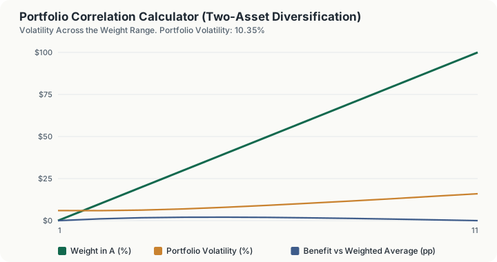
Quick Answer: At the default inputs -- a 60/40 mix of an asset with 16% annual volatility and an asset with 6%, correlated at 0.20 -- portfolio volatility is 10.35%. The weighted average of the two volatilities is 12.00%, so correlation below one removes 1.65 percentage points of risk for free. The minimum-variance mix for this pair holds just 6.62% in the volatile asset and lands at 5.91% volatility, less than either asset held alone.

Overview

Diversification is not the observation that owning two things is safer than owning one. It is a specific arithmetic fact: portfolio volatility is a square-root function of the weights, while portfolio return is a straight line in them. That curvature is the whole benefit, and correlation is the parameter that controls how much of it there is.

This calculator computes the volatility of a two-asset portfolio from three numbers you supply -- each asset's volatility, the weight in the first, and the correlation between them -- and reports the gap between that figure and the weighted average of the two volatilities. The weighted average is what risk would be if the two assets moved in perfect lockstep. Everything below it is the diversification benefit.

It also solves for the minimum-variance mix, the single pair of weights with the lowest achievable volatility, and states whether that mix is calmer than simply owning the safer asset on its own. It often is, which is the counterintuitive result that makes the mathematics worth doing.

Optionally the correlation and both volatilities can be derived from five paired annual returns instead of typed in. The default is off: the fields drive the answer, and the return series is displayed for reference only.

How This Is Calculated

Portfolio variance for two assets is the standard quadratic form:

\sigma_p^2 = w_A^2\sigma_A^2 + w_B^2\sigma_B^2 + 2 w_A w_B \rho \sigma_A \sigma_B

Volatility is its square root. The third term is the only place correlation appears, and it is the only term that can be reduced without changing the assets.

Step 1 -- Convert the volatilities to decimals. 16% becomes 0.16, 6% becomes 0.06

Step 2 -- Set the weights. Weight in A = 0.60, so weight in B = 1 - 0.60 = 0.40

Step 3 -- Compute the covariance. 0.20 x 0.16 x 0.06 = 0.00192

Step 4 -- The first variance term. 0.60² x 0.16² = 0.36 x 0.0256 = 0.009216

Step 5 -- The second variance term. 0.40² x 0.06² = 0.16 x 0.0036 = 0.000576

Step 6 -- The cross term. 2 x 0.60 x 0.40 x 0.00192 = 0.0009216

Step 7 -- Add them. 0.009216 + 0.000576 + 0.0009216 = 0.0107136

Step 8 -- Take the square root. $\sqrt{0.0107136}$ = 0.103507 = 10.35%

Step 9 -- Compute the weighted average volatility for comparison. (0.60 x 16%) + (0.40 x 6%) = 9.6% + 2.4% = 12.00%

Step 10 -- The diversification benefit is the gap. 12.00% - 10.35% = 1.65 percentage points

Step 11 -- The diversification ratio is the quotient. 12.00 / 10.35 = 1.159x

Step 12 -- Solve for the minimum-variance weight. Differentiating the variance with respect to the weight and setting it to zero gives

w_A^* = \frac{\sigma_B^2 - \text{cov}}{\sigma_A^2 + \sigma_B^2 - 2\,\text{cov}}

(0.0036 - 0.00192) / (0.0256 + 0.0036 - 0.00384) = 0.00168 / 0.02536 = 0.0662, or 6.62% in Asset A

The result is clamped into the range 0 to 1, so no short position is ever reported.

Step 13 -- Evaluate volatility at that weight. Running the same variance formula at 6.62% / 93.38% gives 5.91%, which is below the 6.00% of Asset B held alone. That is what the "beats both assets" line is testing.

Worked Example

You hold a 60/40 portfolio. The growth sleeve has run at 16% annualised volatility, the defensive sleeve at 6%, and the two have correlated at about 0.20.

Step 1 -- What you would expect if the two moved together. 12.00%. This is the honest null hypothesis: it is the risk you would carry if correlation were 1.

Step 2 -- What you actually carry. 10.35%

Step 3 -- What correlation bought you. 12.00% - 10.35% = 1.65 percentage points of volatility, at no cost in expected return.

That is the only free lunch in the subject, and it is small. A 1.65 point reduction on a 12 point base is a 13.7% cut in risk. Real, worth having, and nothing like the protection people assume a bond sleeve provides.

Step 4 -- Test the assumption that keeps it. Set the correlation to 1.00. Portfolio volatility becomes exactly 12.00% and the benefit becomes zero. This is not a hypothetical: correlations across risk assets have converged in the middle of several liquidation events, and the diversification vanished precisely when it was needed.

Step 5 -- Find the calmest possible mix. 6.62% in Asset A, at 5.91% volatility. Holding a small slice of the volatile asset is less risky than holding none of it, because at a correlation of 0.20 that slice partly offsets the moves of the other. This is the result that surprises people, and it falls straight out of the derivative.

Step 6 -- Note what the minimum-variance mix does not say. It is a risk optimum only. It contains no expected returns and therefore no claim that you should hold it. A portfolio at 5.91% volatility with 93% in a low-returning asset is calm and may well be inadequate.

What This Does Not Account For

Expected returns. This page computes risk and nothing else. The minimum-variance mix is not a recommendation, and no Sharpe ratio, efficient frontier point or optimal portfolio is produced here.
More than two assets. The formula is the two-asset case. A real portfolio needs a full covariance matrix, and adding a third asset is not a matter of averaging pairs.
Unstable correlations. The correlation is a single fixed number you supply. Correlations move, and they have historically moved most in the direction that hurts, rising toward one during severe drawdowns.
Non-normal returns. Volatility is a standard deviation. It weights a 20% gain and a 20% loss identically and says nothing about skew, fat tails, or the shape of a drawdown.
Any authority for the inputs. The 16%, 6% and 0.20 defaults are illustrative round numbers chosen because they are near long-run figures for broad equity and investment-grade bond indices. They are not a quote, a forecast, or a sourced estimate.
Rebalancing, costs and taxes. The weights are treated as fixed. Nothing models the drift between rebalances or what restoring them costs.
Sampling error in the derived statistics. When the return-series option is switched on, five observations produce a correlation with an extremely wide confidence interval. The figure is arithmetically correct and statistically almost meaningless at that sample size.

Common Pitfalls

Confusing correlation with beta. They answer different questions. Correlation is scale-free and bounded at plus and minus one; beta carries the ratio of the volatilities and is unbounded. On the default return series the correlation is -0.8258 while the beta of B on A is -0.2038. Both are shown so the difference is visible.
Assuming low correlation means low risk. Correlation controls only the cross term. Two assets at 40% volatility with a correlation of zero still make a very volatile portfolio.
Estimating correlation from too little data. Five annual observations, the default series here, is not enough to distinguish a correlation of -0.8 from one of -0.3 with any confidence.
Treating the historical correlation as the forward one. The number that matters is the correlation during the next drawdown, and it is routinely higher than the full-sample figure.
Reading the minimum-variance mix as an allocation. It optimises one thing and ignores return entirely.
Mixing frequencies. A monthly volatility and an annual one cannot be combined. Annualise both before entering them, and use the same period for the correlation.

Frequently Asked Questions

Why is portfolio volatility lower than the weighted average of the two volatilities?

Because volatilities do not add. Variances add, with a cross term scaled by the correlation. Only when the correlation is exactly 1.00 does the square root of the summed variance equal the weighted average of the volatilities. At any lower correlation the portfolio sits below that line, and the gap is the entire diversification benefit: 1.65 percentage points at the defaults here.

Can the minimum-variance portfolio really be safer than the safest asset?

Yes, and it usually is unless the correlation is high. At the defaults the safe asset alone runs at 6.00% volatility while a 6.62/93.38 mix runs at 5.91%. The small allocation to the volatile asset partly cancels the moves of the other. The effect disappears as correlation rises toward one, and grows as it falls toward minus one.

What correlation should I use?

Whatever you can defend, measured over a period relevant to your holding horizon and at the same frequency as your volatilities. Be aware that the answer is unstable: pairs that diversified reliably for a decade have converged inside a single quarter. Running the calculator at a correlation of 1.00 is the most useful stress test on this page, because it shows exactly how much of your risk reduction is an assumption rather than a property of the assets.

What is the difference between the diversification benefit and the diversification ratio?

The benefit is a subtraction, in percentage points: 12.00% minus 10.35% is 1.65 points. The ratio is a division: 12.00 divided by 10.35 is 1.159x. The first tells you how much volatility you removed, the second tells you the proportion by which the weighted average exceeds actual risk. Both come from the same two numbers.

Does the return series option change the headline?

Only if you switch it on. By default the volatilities and correlation come from the fields, and the five paired returns are computed and displayed but do not feed the portfolio calculation. The page states which source was used. With the option on, both volatilities are recomputed as sample standard deviations using the n-1 denominator, and the correlation is taken from the same five pairs.

Does a negative correlation guarantee a profit?

No. It reduces variance, which is a statement about the dispersion of outcomes and not about their average. A portfolio of two negatively correlated assets that both lose money is a smooth path to a loss.

Sources

Markowitz, H., "Portfolio Selection," Journal of Finance, 1952. The origin of the two-asset variance formula and of the minimum-variance solution used here.
The engine implements the standard quadratic form for two-asset variance and the closed-form minimum-variance weight; correlation and the ordinary least squares slope are computed by the platform's shared statistics primitive using the sample (n-1) convention.

Portfolio Correlation Calculator (Two-Asset Diversification)

Assumptions

Preset scenarios

Volatility Across the Weight Range

Portfolio Volatility by Weight in Asset A