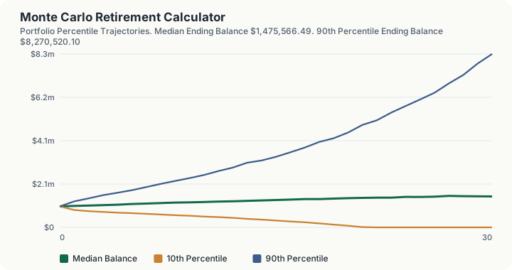
Quick Answer: A $1,000,000 portfolio drawing $40,000 in year one, inflating at 2.5%, survives thirty years in 74.66% of 5,000 simulated paths at a 7% mean return and 15% volatility. 1,267 paths ran out of money, the earliest in year 11. The median ending balance is $1,475,566.49, but the 10th percentile ending balance is $0.
What does this calculator do?
A Monte Carlo retirement projection answers a question a single average-return spreadsheet cannot: not "what happens if returns average 7%", but "across thousands of possible return sequences averaging 7%, how often does the money last?" Those are different questions, and the gap between them is sequence-of-returns risk. A retiree drawing an inflating income is selling assets every year, so a bad decade at the start does damage that a good decade later cannot undo, even when the long-run average is identical.
This simulation is deterministic by design, and that is a deliberate choice worth understanding. The random number generator is seeded explicitly at 2026 and 5,000 paths are run, both pinned in the calculator's configuration and asserted by its test vectors. The seed is not drawn from the clock. The consequence is that identical inputs always produce an identical success rate, to the digit: refreshing this page will never change your answer, and neither will running it tomorrow. A Monte Carlo tool whose headline number wobbles between page loads cannot be checked, cannot be cited, and cannot be trusted by a reader who reloads it.
What is not authoritative is the capital-market assumptions. The 7% mean return, 15% volatility and 2.5% withdrawal inflation are stated assumptions, not published figures, and every one of them is yours to change. The historical bootstrap engines resample a 30-year annual return series carried in the engine; that series is historical data, not a forecast either.
How is this calculated?
Each path steps forward one year at a time. The return is applied first, then the withdrawal is taken at the end of the year, then the withdrawal is inflated for the next year:
Bₜ = B_(t − 1) × (1 + rₜ) − Wₜ; W_(t + 1) = Wₜ × (1 + i)
Under the lognormal engine each year's return is drawn from a seeded standard normal by Box-Muller and transformed:
rₜ = e^((μ − σ²/2) + σzₜ) − 1
Step 1: Compute the drift term once, since the median of a lognormal sits below its mean. 0.07 - (0.5 x 0.15 x 0.15) = 0.07 - 0.01125 = 0.05875
Step 2: Start each path at the portfolio value. $1,000,000, with a first-year withdrawal of $40,000
Step 3: Draw one year's return, apply it, then take the withdrawal. For a path drawing a median return in year one, the return is e^0.05875 - 1 = 6.05%. $1,000,000 x 1.0605 - $40,000 = $1,020,500
Step 4: Inflate the withdrawal for the following year. $40,000 x 1.025 = $41,000
Step 5: Mark a path failed the moment the balance reaches zero or below. A failed path is held at zero for every remaining year and is never resurrected by a later good return.
Step 6: Repeat for 30 years, then repeat the whole path 5,000 times from the same seeded stream.
Step 7: Count the survivors and divide. This is the headline. (5,000 - 1,267) / 5,000 = 3,733 / 5,000 = 74.66%
Step 8: The complement is the failure rate. 100% - 74.66% = 25.34%
Step 9: Sort the 5,000 ending balances and read off the percentiles. 10th percentile: $0 50th percentile: $1,475,566.49 90th percentile: $8,270,520.10
Step 10: Note when failures start. The earliest year in which any path exhausted the portfolio was year 11.
Step 11: Compute the initial withdrawal rate. $40,000 / $1,000,000 = 4%
Step 12: Re-run the entire simulation with the withdrawal cut 10%, against the identical market paths. $40,000 x 0.9 = $36,000 a year, giving a success rate of 81.22%
Step 13: Difference the two success rates. 81.22% - 74.66% = 6.56 percentage points bought by a 10% spending cut
That last step is the most useful number on the page, because it holds the market draws fixed and isolates the one lever you actually control.
Worked Example
A retiree with exactly $1,000,000 wants to spend $40,000 in her first year, rising with 2.5% inflation, for thirty years. She assumes a 7% mean nominal return and 15% volatility, which is roughly a global equity portfolio.
Step 1: Her withdrawal rate. $40,000 / $1,000,000 = 4%, the canonical rule-of-thumb figure.
Step 2: Her success rate. 74.66%. Roughly one path in four fails.
Step 3: How many failed and when. 1,267 of 5,000 paths ran out, the earliest in year 11, which is early enough to matter to a 65-year-old.
Step 4: What the middle outcome looks like. A median ending balance of $1,475,566.49, or nearly half as much again as she started with.
Step 5: What the downside looks like. A 10th percentile ending balance of $0. The distribution is heavily right-skewed, so the median tells you almost nothing about the risk. The 90th percentile of $8,270,520.10 is a reminder that the average outcome is dragged upward by paths she cannot count on.
Step 6: What spending less buys her. Cutting the withdrawal to $36,000 against the identical market paths raises success to 81.22%, a gain of 6.56 percentage points. A 10% spending cut usually does more work than any plausible change in asset allocation, and unlike returns it is entirely within her control.
Step 7: What the number does not say. A 74.66% success rate is not a 74.66% chance of running out being fine. It is a count of paths that survived a rigid, inflation-adjusted withdrawal with no adjustment ever made, no matter how badly the portfolio performed. Real retirees adjust.
Carrying The Distribution Across The Thirty Years
Step 8: Year one. Median $1,022,716, 10th percentile $829,942, 90th percentile $1,240,225. A band of about $410,000 after a single year.
Step 9: Year eleven, the earliest failure. Median $1,231,235, 10th percentile $490,284, 90th percentile $2,685,955. The median is above where she started while the bottom decile has lost more than half.
Step 10: Year twenty-one. Median $1,408,109, 10th percentile $12,727, 90th percentile $4,888,335. The bottom decile is one year from zero.
Step 11: Year thirty. Median $1,475,566, 10th percentile $0, 90th percentile $8,270,520
The median line is almost flat across thirty years, drifting from $1.00m to $1.48m, while the band around it opens from $410,000 to more than $8.2m. Nothing useful about this retirement is in the middle line. The whole decision sits in how fast the bottom decile falls away, and that is visible by year eleven.
What does this calculator not account for?
- Spending flexibility of any kind. Withdrawals inflate every year regardless of portfolio performance. There are no guardrails, no spending cuts in bad years, and no discretionary versus essential split. Real retirees cut back, and doing so raises success substantially, as step 13 shows.
- Taxes. Withdrawals are gross. No account is made for the tax character of the assets, required minimum distributions, or the difference between a taxable account, a traditional IRA and a Roth.
- Social Security, pensions and annuities. Any guaranteed income floor would reduce the portfolio withdrawal and change the answer substantially.
- Fees. The return you enter is treated as net. Fund expenses and advisory fees are not deducted separately.
- Changing asset allocation over time. A single mean and volatility apply for the whole horizon. Glide paths are not modelled.
- Fat tails and correlation. The lognormal engine draws each year independently, which never produces the multi-year crash runs that history contains. That is exactly why the block bootstrap engine exists: it resamples consecutive historical years and preserves those runs.
- Longevity uncertainty. The horizon is a fixed number of years you choose, not a mortality distribution.
What mistakes do people make with this?
- Reading the success rate as a probability of a good retirement. It is the share of rigid, never-adjusted paths that survived. Treat it as a stress-test score, not a forecast.
- Planning against the median. The median ending balance is $1,475,566.49 and the 10th percentile is $0. The distribution is so skewed that the median is a poor guide to anything. Plan against the 10th percentile.
- Reading a large 90th percentile as success. Very large surpluses usually mean you underspent for thirty years, not that the plan was well designed.
- Assuming more simulations means more accuracy. Beyond a few thousand paths the sampling noise is small compared with the error in the return and volatility assumptions themselves. Changing the mean return by half a point moves the answer far more than changing the path count.
- Trusting the lognormal engine on crash risk. Independent annual draws systematically understate multi-year drawdowns. Run the block bootstrap engine as a cross-check.
- Being surprised that the number never changes. That is the design. The seed is pinned at 2026 so the result is reproducible; the stability is a feature, not a sign that the simulation is not running.
Frequently Asked Questions
What is a good Monte Carlo success rate for retirement?
Why does the answer never change when I reload the page?
Does the 4% rule work?
What is the difference between the three return engines?
Where do the 7% return and 15% volatility come from?
Why is the 10th percentile ending balance zero?
Sources
- Metropolis, N. and Ulam, S. (1949), "The Monte Carlo Method," Journal of the American Statistical Association 44(247). doi.org/10.1080/01621459.1949.10483310
- Milevsky, M. A. and Robinson, C. (2005), "A Sustainable Spending Rate without Simulation," Financial Analysts Journal 61(6). doi.org/10.2469/faj.v61.n6.2776
Also consulted: No statutory or published data source underlies this page. The mean return, volatility, withdrawal inflation, portfolio value, withdrawal amount and horizon are all user-supplied assumptions with no authority behind their defaults; The simulation engine is documented in engine/primitives/montecarlo.ts: a Mulberry32 seeded pseudo-random generator, standard normals by Box-Muller, geometric Brownian motion with drift mu minus one half sigma squared, returns applied before an end-of-year withdrawal, and failed paths held at zero. The seed of 2026 and the 5,000-path count are pinned in the calculator's own configuration; The historical bootstrap engines resample a 30-year annual return series carried in the same primitive.