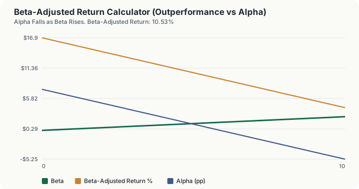
Quick Answer: A portfolio returning 11.8% against a benchmark that returned 9.4%, with a beta of 1.25 and a 4.3% risk-free rate, has a beta-adjusted return of 10.53%. The raw 2.40 percentage points of outperformance splits into 1.28 points bought with extra market exposure and 1.13 points of genuine alpha, so beta explains 53.1% of the gap.
What does this calculator do?
Every factsheet leads with the same number: the portfolio return minus the benchmark return. It is the least informative statistic in performance measurement, because it says nothing about how much market risk was taken to produce it.
A manager who runs at a beta of 1.25 has, by construction, 25% more exposure to the index than the index itself. In a rising market that alone produces outperformance, and it required no skill whatsoever: anyone could have bought the same exposure with a cheap leveraged index position. The question worth asking is what is left after paying for that exposure at the market's own price.
This calculator answers it using an identity that holds exactly for any set of inputs:
Rₚ − Rₘ = (β − 1)(Rₘ − R_f) + α
The gap against the benchmark decomposes without residual into a beta-explained component and Jensen's alpha. Nothing is estimated and nothing is approximated; the two pieces always sum to the whole. That is what makes the split usable as an argument rather than as an opinion.
The page reports the same record across a ladder of betas from 0 to 2.50, holding the returns fixed, so you can see the beta level at which the record stops being impressive. It also reports that crossover directly: the beta above which this performance becomes negative alpha.
How is this calculated?
E(R) = R_f + β(Rₘ − R_f); α = Rₚ − E(R)
Beta-explained = (β − 1)(Rₘ − R_f); R_(β -adj) = Rₚ − (β − 1)(Rₘ − R_f)
Step 1: Compute the CAPM required return. The risk-free rate plus beta multiplied by the benchmark's excess return over the risk-free rate. This is the bar the portfolio had to clear before anything counts as skill.
Step 2: Compute alpha as the residual. Portfolio return less that required return. This is Jensen's alpha, in percentage points.
Step 3: Compute raw outperformance. Portfolio return less benchmark return, with no risk adjustment at all.
Step 4: Compute the beta-explained component. Beta minus one, multiplied by the benchmark's excess return. At a beta of exactly 1.00 this term is zero, which is why alpha and raw outperformance coincide there.
Step 5: Strip the beta component out of the reported return. Portfolio return less the beta-explained component. That is the headline beta-adjusted return, and it is algebraically equal to the benchmark return plus alpha.
Step 6: Express beta's share of the gap. The beta-explained component divided by the raw gap. This is reported as "N/A" when the raw gap is exactly zero, because the ratio is then undefined.
Step 7: Solve for the breakeven beta. The calculator reports the beta at which alpha turns negative, computed as one plus the raw gap divided by the benchmark's excess return. Above it, this record has negative alpha.
Step 8: Rebuild the decomposition across betas. The table repeats steps 1 to 5 for eleven betas from 0.00 to 2.50 in steps of 0.25, holding all three returns fixed.
The verdict line is chosen from four cases by the signs of alpha, the raw gap and the beta component: beat the index with alpha intact, beat it with leverage explaining all of it, lagged it but still added alpha, or lagged on both bases.
Worked Example
Defaults: portfolio 11.8%, benchmark 9.4%, risk-free 4.3%, beta 1.25.
Step 1: Find the benchmark's excess return, which is the price of one unit of beta. 9.4% − 4.3% = 5.10 percentage points
Step 2: Find the CAPM required return at this beta. 4.3% + (1.25 × 5.10%) = 4.3% + 6.375% = 10.68%
Step 3: Find alpha. 11.8% − 10.675% = 1.13 percentage points
Step 4: Find the raw outperformance the factsheet would report. 11.8% − 9.4% = 2.40 percentage points
Step 5: Find how much of that gap the extra beta explains. (1.25 − 1.00) × 5.10% = 0.25 × 5.10% = 1.28 percentage points
Step 6: Check the identity closes. 1.275 + 1.125 = 2.40 percentage points, the whole gap
Step 7: Compute the beta-adjusted return. 11.8% − 1.275% = 10.53%
Step 8: Express beta's share of the outperformance. 1.275 ÷ 2.40 = 53.1%
Step 9: Find the beta at which this record would have no alpha left. 1 + (2.40 ÷ 5.10) = 1.47
So slightly more than half of the headline outperformance was market exposure. The manager still added 1.13 points of value, but had the same returns been produced at a beta of 1.60 rather than 1.25, alpha would have been negative and the outperformance would have been an artefact of leverage.
What does this calculator not account for?
- Beta is an input, not an estimate. The calculator does not regress anything. You supply beta, and the answer inherits every weakness of however it was measured: window length, return frequency, and the benchmark it was measured against.
- A single period, single benchmark, single factor. There is no multi-factor attribution here: no size, value, momentum, quality or profitability factor. Alpha in this model is everything CAPM cannot explain, which in practice includes exposures that have known prices.
- No statistical significance. One period of alpha is not evidence of skill. The calculator produces a point estimate with no standard error, no t-statistic and no sample size.
- No compounding or period alignment. All four inputs are treated as simple annualised percentages over the same period. Nothing chain-links sub-period returns.
- Fees, taxes, and trading costs. Enter returns already net of whatever you want measured; the calculator applies nothing.
- A time-varying beta. A portfolio that shifted exposure through the period has one beta here, and the decomposition treats it as constant.
- The inputs have no authority. Risk-free rate, benchmark return and beta are yours to choose. Nothing in this page is sourced from a market data provider, and no default should be read as a recommendation.
What mistakes do people make with this?
Measuring beta against a different index than you benchmark to. The identity holds only when the beta and the benchmark refer to the same index. A beta measured against a broad market index but compared against a sector benchmark produces a decomposition that means nothing.
Reading a positive alpha as skill. Alpha is a residual. It absorbs mismeasured beta, factor exposures, illiquidity premia and luck. Positive alpha means the return exceeded what one factor could explain, not that a person earned it.
Forgetting the risk-free rate matters. Beta scales the excess return, not the whole return. At a benchmark return of 9.4% and a risk-free rate of 4.3%, one unit of beta buys 5.10 points, not 9.4. Using zero as the risk-free rate would nearly double the beta-explained figure.
Assuming a low-beta laggard failed. A portfolio can trail its index and still have added value. At a beta of 0.70 a portfolio returning 8.2% against the same 9.4% benchmark has positive alpha, because CAPM only required 7.87%.
Comparing beta-adjusted returns across different benchmarks. The figure is defined relative to one index and one risk-free rate. Two managers on different benchmarks cannot be ranked on it.
Frequently Asked Questions
What is the difference between alpha and beta-adjusted return?
Why is my beta-adjusted return lower than my actual return?
At a beta of 1.0, why do alpha and raw outperformance agree?
What beta would make my outperformance disappear?
Can a portfolio that lagged the index still have positive alpha?
Is Jensen's alpha the same thing as excess return?
Sources
- U.S. Securities and Exchange Commission, Investor.gov, the official authority for the investing this calculator relates to. investor.gov
Also consulted: CAPM required return: E(Rᵢ) = R_f + βᵢ(E(Rₘ) − R_f); Jensen's alpha: portfolio return less the CAPM required return; The decomposition identity Rₚ − Rₘ = (β − 1)(Rₘ − R_f) + α, which follows from substituting the CAPM expression into the definition of alpha and holds exactly for all inputs; Portfolio return, benchmark return, risk-free rate and beta are all user inputs with no authoritative source. The defaults are illustrative only.
This page contains no statutory or published data. The decomposition is pure arithmetic implemented in engine/primitives/returns.ts (alphaDecomposition, capmExpectedReturn) and covered by golden vectors.