Sharpe Ratio Calculator

The Sharpe Ratio, developed by Nobel laureate William F. Sharpe in 1966, is the most widely used single number for comparing investments on a risk-adjusted basis. Raw returns alone are misleading: a portfolio that returned 15% by taking on wild, unpredictable swings is not obviously better than one that returned 10% smoothly and predictably. The Sharpe Ratio answers the question those raw numbers cannot: for the amount of volatility an investor had to tolerate, how much extra return did they actually get paid for taking it?

The formula starts with excess return, the portfolio's return minus the return available from a risk-free asset like a Treasury bill, since that risk-free return represents the baseline any investor could earn without taking on market risk at all. It then divides that excess return by the portfolio's standard deviation, a standard statistical measure of how much returns fluctuate around their average. A higher Sharpe Ratio means more excess return per unit of volatility, which is generally the more desirable outcome for a risk-averse investor. A Sharpe Ratio of 1.0 is often considered a reasonable baseline, 2.0 or higher is considered very good, and 3.0 or higher is considered excellent, though these thresholds shift with market conditions and are more meaningful as a comparison across similar strategies than as absolute pass/fail marks.

Because it uses standard deviation, the Sharpe Ratio treats upside and downside volatility identically, penalizing a fund for large positive swings just as much as large negative ones. This is a deliberate simplification that makes the metric easy to compute and compare, but it is also the source of its best-known criticism, addressed by variants like the Sortino Ratio, which counts only downside volatility.

The Sharpe Ratio formula is:

$$\text{Sharpe Ratio} = \frac{R_p - R_f}{\sigma_p}$$

Where $R_p$ is the portfolio's return over the measurement period, $R_f$ is the risk-free rate over the same period, and $\sigma_p$ is the standard deviation of the portfolio's periodic returns, both measured over consistent, matching timeframes (both annualized, or both monthly, for example).

This calculator computes the Sharpe Ratio using the platform's dedicated calculateSharpeRatio primitive, which implements this exact formula on arbitrary-precision Decimal values. It also derives a secondary, explicitly illustrative figure: treating the Sharpe Ratio itself as a z-score under the simplifying assumption that annual returns are normally distributed, it estimates the approximate probability that the portfolio's return will exceed the risk-free rate in a given year, using the standard normal cumulative distribution function. This probability estimate is a rough, assumption-heavy illustration of what the Sharpe Ratio implies statistically, not a rigorous forecast, since real portfolio returns are rarely perfectly normally distributed.

Consider a portfolio with the following annualized figures for the measurement period:

• Portfolio Return ($R_p$): 12.0%
• Risk-Free Rate ($R_f$): 4.5% (approximating a 3-month Treasury bill yield)
• Portfolio Standard Deviation ($\sigma_p$): 15.0%

Step 1: Excess return. $$R_p - R_f = 12.0\% - 4.5\% = 7.5\%$$

Step 2: Sharpe Ratio. $$\text{Sharpe Ratio} = \frac{7.5\%}{15.0\%} = 0.50$$

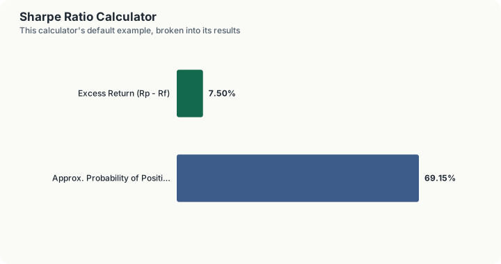
A Sharpe Ratio of 0.50 falls into the "suboptimal" range under common qualitative bands, meaning the portfolio earned some excess return above the risk-free rate but at a relatively high cost in volatility relative to that excess return. Treating 0.50 as an approximate z-score and applying the standard normal cumulative distribution function suggests roughly a 69% probability of a positive excess return in a typical year under a normal-distribution assumption, an illustrative figure rather than a precise forecast.

The Sharpe Ratio's core assumption, that standard deviation is an adequate measure of "risk," breaks down for return distributions that are not roughly normal, which describes many real-world strategies. Portfolios that use options, sell insurance-like exposures, or otherwise generate returns with fat tails or significant skew can show an attractive Sharpe Ratio while carrying meaningful hidden downside risk that standard deviation understates. The ratio penalizes upside volatility exactly as much as downside volatility, which can unfairly punish strategies with large, infrequent positive outcomes. It is highly sensitive to the measurement period and the choice of risk-free rate; a Sharpe Ratio calculated over a strong bull market will typically look very different from one calculated over a full market cycle including a drawdown. It also says nothing about the magnitude of maximum drawdown an investor might have had to endure to earn that risk-adjusted return, which matters enormously for real-world investor behavior and the risk of forced or panic-driven selling.

• Comparing Sharpe Ratios calculated over different time periods or frequencies. A Sharpe Ratio computed from monthly returns is not directly comparable to one computed from annual returns without proper annualization (typically scaling by the square root of the number of periods per year).
• Using a risk-free rate that does not match the measurement period. Pairing a long-dated Treasury yield with a short measurement window, or vice versa, introduces a mismatch that distorts the excess return figure.
• Treating a high Sharpe Ratio as proof of skill rather than a description of one period's results. Sharpe Ratios calculated over short or unusually calm periods can look inflated and may not persist.
• Applying the Sharpe Ratio to strategies with non-normal return distributions without caveat. Strategies involving options, leverage, or illiquid assets often have return patterns where standard deviation understates true tail risk.
• Ignoring negative Sharpe Ratios as simply "bad" without context. A negative Sharpe Ratio during a broad market downturn may still represent relative outperformance versus peers who fared worse; always compare against an appropriate benchmark.

• Sharpe, William F. "Mutual Fund Performance." Journal of Business, 1966.
• Sharpe, William F. "The Sharpe Ratio." Journal of Portfolio Management, 1994.
• CFA Institute. Portfolio Risk and Return: Part II, CFA Program Curriculum.
• U.S. Department of the Treasury. Daily Treasury Par Yield Curve Rates (risk-free rate reference data).