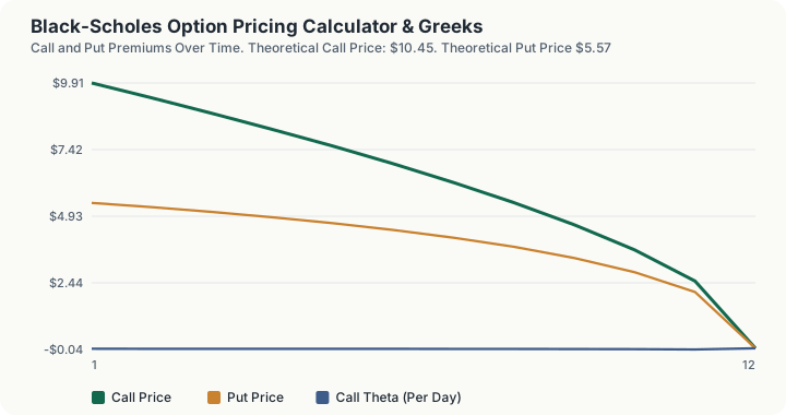
Quick Answer: For an at-the-money option with a $100 stock, $100 strike, one year to expiry, 20% implied volatility, and a 5% risk-free rate, the Black-Scholes model prices the call at $10.45 and the put at $5.57, with a call delta of 0.637.
Overview
The Black-Scholes model is the closed-form equation Fischer Black, Myron Scholes, and Robert Merton published in the early 1970s for pricing European-style options, options that can only be exercised at expiration, not before. It remains the reference point for options pricing across trading desks and retail platforms alike, not because real markets perfectly match its assumptions, but because it gives a fast, mathematically consistent baseline that every other pricing approach gets compared against.
This calculator implements the full closed-form model: call and put prices, both d1 and d2, and the five standard Greeks (delta, gamma, theta, vega, and rho) for the call side, computed directly from the same formula published in the original paper. There is no numerical approximation or lattice method involved; every output is an exact evaluation of the Black-Scholes-Merton equations given the five inputs you provide.
How This Is Calculated
The model prices a European call or put as a function of five inputs: the underlying price ($S$), the strike price ($K$), time to expiration in years ($T$), the risk-free rate ($r$), volatility ($\sigma$), and, in the extended Merton form used here, a continuous dividend yield ($q$).
Step 1: Compute d1 and d2.
$d_1$ and $d_2$ are the standardized distances (in units of volatility-adjusted standard deviations) that the log of the stock price is expected to travel relative to the strike by expiration, under the model's risk-neutral assumptions.
Step 2: Price the call and put using the cumulative standard normal distribution N(x).
$N(d_2)$ can be read as the risk-neutral probability the option finishes in the money, and $N(d_1)$ is the delta-weighted probability used to value the underlying's contribution to the payoff.
Step 3: Derive the Greeks by differentiating the pricing formula. Delta measures price sensitivity to a $1 move in the underlying, gamma measures how fast delta itself changes, vega measures sensitivity to a 1-point change in implied volatility, theta measures the dollar value lost per day purely from time passing, and rho measures sensitivity to a 1% change in the risk-free rate. Each is computed from the closed-form partial derivative of the pricing equation, not estimated numerically.
Key assumptions baked into the model: the underlying follows geometric Brownian motion with constant volatility, the risk-free rate and volatility are constant over the option's life, markets have no transaction costs or arbitrage opportunities, the underlying can be traded continuously, and the option is European (exercisable only at expiration).
Worked Example
Using this calculator's own baseline inputs:
- Underlying price: $100
- Strike price: $100
- Time to expiration: 365 days (1.00 year)
- Implied volatility: 20%
- Risk-free rate: 5%
- Dividend yield: 0%
Step by step: $\ln(100/100) = 0$, so $d_1 = \frac{0 + (0.05 - 0 + 0.5 \times 0.2^2)(1)}{0.2\sqrt{1}} = \frac{0.07}{0.2} = 0.3500$, and $d_2 = 0.3500 - 0.2000 = 0.1500$. Looking up the standard normal CDF: $N(d_1) = 0.6368$ and $N(d_2) = 0.5596$.
Call price = $100 \times 0.6368 - 100 \times e^{-0.05} \times 0.5596 = 63.68 - 53.23 = $$10.45. Put price = $100 \times e^{-0.05} \times (1 - 0.5596) - 100 \times (1 - 0.6368) = 41.89 - 36.32 = $$5.57. Both match this calculator's own baseline test vectors.
The Greeks at this same point: call delta ≈ 0.637 (the call gains about 64 cents for every $1 the stock rises), gamma ≈ 0.0188 (delta itself shifts by about 0.0188 per $1 move), vega ≈ 0.375 (the call gains about 37.5 cents for every 1-percentage-point rise in implied volatility), daily theta ≈ −$0.018 (the option loses about 1.8 cents in value per day purely from time decay, holding everything else constant), and rho ≈ 0.532 (the call gains about 53 cents for every 1-percentage-point rise in the risk-free rate). Switching to the "Elevated Volatility (40% IV)" scenario roughly doubles vega's dollar impact and pushes both call and put prices meaningfully higher, since higher volatility increases the value of optionality in both directions.
What This Does Not Account For
- American-style early exercise. Black-Scholes prices European options only. American options, especially dividend-paying stocks' calls or deep in-the-money puts, can be worth more due to the early exercise right, which this model does not price.
- Volatility skew and smile. Real options markets price different strikes and expirations with different implied volatilities rather than the single flat volatility this model assumes; a single-input IV here cannot capture that structure.
- Discrete dividends. The model uses a continuous dividend yield ($q$), which is a reasonable approximation for broad indices but less accurate for stocks paying discrete, lumpy dividends around specific ex-dividend dates.
- Transaction costs, bid-ask spreads, and liquidity. The theoretical price ignores the frictional costs of actually entering or exiting a position.
- Jump risk and non-normal returns. Geometric Brownian motion assumes continuous price paths; real markets experience gaps and jumps that this model structurally cannot represent.
Common Pitfalls
- Treating the theoretical price as a market-clearing price. Black-Scholes gives a model price given your inputs; actual quoted option prices reflect supply, demand, and the market's own view of volatility, which may differ from what you entered.
- Using historical volatility instead of implied volatility. The model calls for a forward-looking volatility estimate; plugging in trailing realized volatility can produce a systematically biased price versus what the market is actually quoting.
- Forgetting that theta is not linear. Time decay accelerates as expiration approaches, especially for at-the-money options; the daily theta figure shown here is a snapshot at the current inputs, not a constant daily charge for the life of the option.
- Misreading vega's units. Vega here is scaled per 1 percentage point of volatility (for example, IV moving from 20% to 21%), not per 1.0 (100 percentage points), a common source of order-of-magnitude confusion.
- Applying the model to American options without adjustment. For dividend-paying American calls or most American puts, Black-Scholes systematically misprices relative to models that account for early exercise, such as a binomial tree.
Frequently Asked Questions
What is the difference between d1 and d2?
Why does the put price differ from the call price at the same strike?
Does this calculator handle American-style options?
Can this calculator find the implied volatility from a market option price?
What does a negative theta mean?
How sensitive is the price to the volatility input?
Sources
- Black, F. and Scholes, M. (1973), "The Pricing of Options and Corporate Liabilities," Journal of Political Economy. The original derivation of the option pricing formula used here. doi.org/10.1086/260062
Also consulted: Black, F., and Scholes, M., "The Pricing of Options and Corporate Liabilities," Journal of Political Economy, 1973; Merton, R.C., "Theory of Rational Option Pricing," Bell Journal of Economics and Management Science, 1973 (continuous dividend yield extension); Hull, J.C., "Options, Futures, and Other Derivatives," standard reference text for Greeks derivations; Chicago Board Options Exchange (Cboe), options pricing and Greeks education resources.