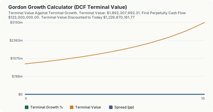
Quick Answer: A final projected free cash flow of $120,000,000, growing at 2.5% forever and discounted at 9%, produces a terminal value of $1,892,307,692.31. Discounted back over the 5 years to the terminal year, that is $1,229,870,161.77 in present value. The whole result rests on a 6.50 point spread between the discount rate and the growth rate, and adding just 50 basis points to growth raises the terminal value by 8.86%.
What does this calculator do?
In a typical discounted cash flow model, the terminal value is most of the answer. The explicit forecast covers five or ten years; the terminal value covers everything after that, which is to say forever. It routinely accounts for two thirds or more of the total valuation, and it is produced by a formula with three inputs and one very sharp edge.
The Gordon growth model collapses that infinite tail into a single figure:
TV = (CF_(n + 1))/(r − g)
The edge is the denominator. Value is proportional to $1/(r-g)$, so the elasticity of value with respect to the spread is exactly −1: halve the spread and you double the value. At a six point spread, 50 basis points of extra growth is worth about 9%. At a one point spread, the same 50 basis points is worth 100%. The assumption that moves the answer most is the one readers skim past fastest.
And past a certain point the model does not merely become aggressive, it stops existing. When growth reaches the discount rate the denominator hits zero and the perpetuity diverges. That is not a very large valuation, it is the absence of one, and this calculator says so rather than returning an infinity or a negative number.
The most useful output on the page is often not the terminal value at all. It is the implied growth rate: the growth the market's own price already assumes. Asking whether that number is credible is usually a better test than asking whether your model output is.
How is this calculated?
CF_(n + 1) = CFₙ × (1 + g); TV = (CF_(n + 1))/(r − g); PV₀ = TV/((1 + r)^y)
g_implied = r − (CF_(n + 1))/P
Step 1: Grow the final projected cash flow by one more period. The Gordon formula discounts CF_(n + 1), not CFₙ. Skipping this step is the single most common error in terminal value work, and it understates the answer by exactly one growth period.
Step 2: Compute the spread. Discount rate less growth rate, reported in percentage points. This is the entire denominator.
Step 3: Test for convergence. If the growth rate is greater than or equal to the discount rate, the calculator returns no value and reports that the model diverges. No infinity, no negative number, no silent nonsense.
Step 4: Divide. The grown cash flow divided by the spread as a decimal. That is the terminal value, expressed in the money of the terminal year.
Step 5: Discount it back to today. The terminal value divided by one plus the discount rate, raised to the number of years until the terminal year. In most DCFs this figure alone is the majority of the total valuation.
Step 6: Compute the implied cash flow yield. The grown cash flow divided by the terminal value. Whenever the model is defined, this equals the spread exactly, which is a useful arithmetic check.
Step 7: Measure the fragility. The calculator recomputes the whole valuation with 50 basis points added to the growth rate, regrowing the base cash flow at the higher rate as well as widening the denominator, and reports the percentage change in value. This is computed only when the discount rate still exceeds the bumped growth rate.
Step 8: Invert against the market price. Discount rate less the grown cash flow divided by the market value you entered. That is the perpetual growth rate the traded price implies.
Step 9: Build the sensitivity ladder. The terminal value is recomputed at eleven growth rates from 0.0% to 5.0% in half-point steps, with the spread shown alongside each, so the curve's steepening is visible rather than merely asserted.
Worked Example
Defaults: $120,000,000 final projected cash flow, 9% discount rate, 2.5% terminal growth, 5 years to the terminal year, $1,500,000,000 market value.
Step 1: Grow the final year's cash flow one more period. $120,000,000 × 1.025 = $123,000,000
Step 2: Compute the spread. 9.0% − 2.5% = 6.50 percentage points, or 0.065
Step 3: Confirm the model converges. 9.0% exceeds 2.5%, so the perpetuity has a finite value: converges
Step 4: Divide to get the terminal value. $123,000,000 ÷ 0.065 = $1,892,307,692.31
Step 5: Discount it back over five years. 1.09^5 = 1.538624, and $1,892,307,692.31 ÷ 1.538624 = $1,229,870,161.77
Step 6: Check the implied yield. $123,000,000 ÷ $1,892,307,692.31 = 6.50%, equal to the spread as it must be
Step 7: Stress the growth assumption by 50 basis points. At 3.0% growth: $120,000,000 × 1.03 = $123,600,000, and $123,600,000 ÷ 0.06 = $2,060,000,000 ($2,060,000,000 − $1,892,307,692.31) ÷ $1,892,307,692.31 = +8.86%
Step 8: Invert the formula against the traded price. $123,000,000 ÷ $1,500,000,000 = 8.20%, and 9.0% − 8.20% = 0.80% implied growth
Step 8 is the sharpest result on the page. Your model assumes 2.5% growth forever and produces a terminal value 26% above the market price. The market, at 9%, is pricing 0.80%. The disagreement is not about arithmetic; it is entirely about whether the business grows at inflation or at less than half of it, and that is a question you can actually argue about.
Step 7 is the warning. Move terminal growth from 2.5% to 8% against the same 9% discount rate and the spread falls to one point: the terminal value multiplies almost sevenfold, from a change most readers would not notice in a model footnote.
What does this calculator not account for?
- The perpetuity itself is the assumption. A single growth rate applied forever is a modelling convention, not a description of any business. Nothing here validates that the firm survives, that the cash flow is normalised, or that competitive advantage persists.
- No sanity ceiling on growth. The calculator accepts terminal growth up to 20%. Any rate above long-run nominal GDP growth implies the firm eventually becomes the entire economy. That is arithmetic, not judgement, but the model will not stop you.
- No exit multiple cross-check. Practitioners normally sanity-check a Gordon terminal value against an EBITDA or earnings multiple. That comparison is not computed here.
- No mid-year convention. The terminal value is discounted as an end-of-period amount over whole years. A mid-year adjustment would raise the present value slightly.
- No explicit forecast period. The calculator values the tail only. The present value of the years before the terminal year is not added, so the discounted figure is the terminal value's contribution alone, not a full enterprise value.
- The discount rate is not derived. WACC, capital structure, cost of debt, tax shields and beta all sit outside this page. You supply $r$.
- No net debt bridge. Nothing converts enterprise value to equity value.
- No reinvestment consistency check. A growth rate should be supported by reinvestment and a return on capital that generate it. The model happily accepts a growth rate with no reinvestment behind it, which is the most common way a terminal value is quietly inflated.
- Every input is your assumption. Cash flow, discount rate, growth rate and market value have no authoritative source. The defaults are illustrative only, and none of this is investment advice.
What mistakes do people make with this?
Forgetting to grow the final cash flow. The numerator is CF_(n + 1), not CFₙ. Dividing the last projected year straight into the spread understates the terminal value by a factor of $(1+g)$: 2.5% here, and more at higher growth rates.
Using a growth rate above long-run nominal GDP. A firm growing perpetually faster than the economy eventually exceeds it. Two to three percent is the defensible range for a mature developed-market business, and figures above that need an explicit argument.
Failing to notice how small the spread is. The whole result is proportional to $1/(r-g)$. A model with a two point spread is not a slightly more optimistic version of one with a six point spread; it is roughly three times the answer.
Presenting a diverged model as a large number. When growth meets or exceeds the discount rate there is no value, not a big one. A spreadsheet returning a negative or astronomically large figure in that case is reporting a division artefact.
Discounting the terminal value by the wrong number of years. It sits at the end of the final explicit forecast year, so it is discounted over that many years: five here, not six.
Reading the model output as more reliable than the price. Terminal value is the least verifiable part of a DCF and usually the largest. Where model and market disagree, the implied growth rate tells you what you would have to believe, which is generally the more honest framing.
Frequently Asked Questions
What is the Gordon growth model used for?
Why do I have to grow the final year's cash flow first?
What terminal growth rate should I use?
What happens if growth equals or exceeds the discount rate?
How sensitive is terminal value to the growth rate?
What does the implied growth rate tell me?
Sources
- Gordon, M. J. (1959), "Dividends, Earnings, and Stock Prices," The Review of Economics and Statistics. The constant-growth valuation model. doi.org/10.2307/1927792
Also consulted: Growing perpetuity: PV = CF_(n + 1)/(r − g), defined only for $r > g$; the primitive raises rather than returning a value when the series diverges, and the calculator surfaces that as a convergence flag; Terminal value discounted to today: TV/(1 + r)^y, where $y$ is the number of years until the terminal year; Implied growth: g = r − CF_(n + 1)/P, the inversion of the same formula against a traded price; Cash flow, discount rate, terminal growth and market value are all user inputs with no authoritative source.
This page contains no statutory or published data. The Gordon growth model is a closed-form result, implemented in engine/primitives/annuities.ts (gordonGrowthValuation, growingPerpetuityPV, impliedGordonGrowthPercent) and covered by golden vectors.