Quick Answer: The Two-Stage Dividend Discount Model estimates a stock's intrinsic value by discounting an initial period of higher-than-normal dividend growth back to today, then adding the discounted value of all dividends that follow once growth settles into a slower, permanent rate.
Overview
The dividend discount model rests on a simple premise: a share of stock is worth the present value of every dividend it will ever pay. The challenge is that a company's dividend growth rate rarely stays constant forever. A young or fast-growing company might grow its dividend at 15% or 20% a year for a while, but that pace is mathematically impossible to sustain indefinitely, since it would eventually exceed the growth of the entire economy. Sooner or later, growth has to slow to something closer to long-run GDP growth or inflation.
The single-stage Gordon Growth Model handles this by assuming one constant growth rate forever, which works reasonably well for mature, slow-growing companies but badly understates the value of a company still in a high-growth phase. The Two-Stage Dividend Discount Model splits the valuation into two distinct periods to fix this: an explicit high-growth stage lasting N years, followed by a terminal stage assumed to grow at a lower, sustainable rate forever after.
This calculator discounts each year of the high-growth stage individually, then values the entire perpetual stable-growth stage as of the end of the high-growth period using the Gordon Growth formula, and finally discounts that lump-sum terminal value back to today alongside the high-growth dividends.
How This Is Calculated
Stage 1: discount each high-growth dividend individually.
For each year t from 1 to N, the dividend paid in that year is:
D_t = D0 × (1 + g1)^t
where D0 is the current annual dividend and g1 is the high-growth rate. Each of these dividends is discounted back to today at the investor's required rate of return, r:
PV(D_t) = D_t / (1 + r)^t
This calculator performs that discounting using solvePV() from the platform's time-value-of-money engine for every single year, rather than a simplified closed-form shortcut, so the exact per-year cash flow is always visible.
Stage 2: value everything after year N as a single terminal value.
Once the company settles into its permanent growth rate g2, the value of all dividends from year N+1 onward, as of the end of year N, is given by the standard Gordon Growth formula:
Terminal Value at Year N = D_(N+1) / (r − g2)
where D_(N+1) = D_N × (1 + g2) is the first dividend of the stable-growth period. This terminal value is itself a future amount, so it must be discounted back to today just like any other year-N cash flow, again using solvePV():
PV(Terminal Value) = Terminal Value at Year N / (1 + r)^N
Combine both stages.
Intrinsic Value = Sum of Stage 1 present values + PV(Terminal Value)
Note that the model requires r to be strictly greater than g2. If the stable growth rate equals or exceeds the discount rate, the Gordon Growth denominator (r − g2) turns zero or negative and the formula returns a nonsensical or infinite value, a well-known limitation of every constant-growth perpetuity model rather than something specific to this calculator. So that the page still returns a finite number instead of failing, the calculator substitutes a discount rate of g2 + 0.1 percentage points whenever you enter an r at or below g2. Treat any result produced that way as meaningless: it reflects the substituted rate, not the one you typed. Lower the stable growth rate or raise the required return until r sits comfortably above g2 before reading the output.
Worked Example
A stock pays a $2.00 annual dividend today, is expected to grow it 15% a year for five years, then settle permanently to 4%. The required return is 9%.
Step 1 -- Project the five high-growth dividends. $2.00 x 1.15 = $2.30, then $2.645, $3.04175, $3.498013 and $4.022714 in year 5
Step 2 -- Discount each one back to today at 9%.
| Year | Dividend | Discount factor | Present value |
|---|---|---|---|
| 1 | $2.300000 | 1.09 | $2.1101 |
| 2 | $2.645000 | 1.09^2 | $2.2265 |
| 3 | $3.041750 | 1.09^3 | $2.3491 |
| 4 | $3.498013 | 1.09^4 | $2.4780 |
| 5 | $4.022714 | 1.09^5 | $2.6146 |
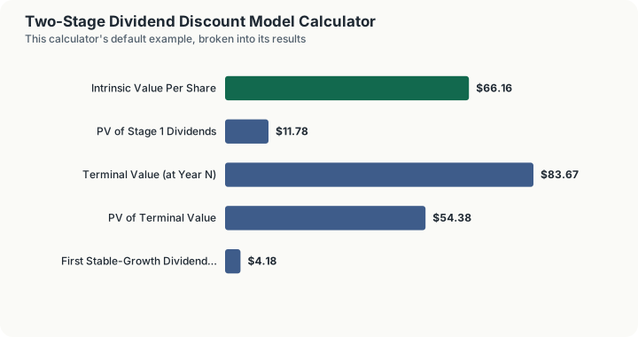
Step 3 -- Sum the stage 1 present values. $2.1101 + $2.2265 + $2.3491 + $2.4780 + $2.6146 = $11.78
Step 4 -- The first stable-growth dividend. $4.022714 x 1.04 = $4.18
Step 5 -- Terminal value at the end of year 5. $4.18 / (0.09 - 0.04) = $4.18 / 0.05 = $83.67
Step 6 -- Discount the terminal value back five years. $83.67 / 1.09^5 = $54.38
Step 7 -- Intrinsic value per share. $11.78 + $54.38 = $66.16
Step 8 -- How much of the value lives in the terminal stage. $54.38 / $66.16 = 82.2%
Step 8 is the honest health warning on every two-stage DDM. Five years of explicitly modelled dividends account for less than a fifth of the answer; the rest is a single perpetuity formula resting on two assumptions about the indefinite future. All the analytical effort usually goes into stage 1, and almost all the valuation comes from stage 2.
What the terminal assumptions are actually worth
Step 9 -- Raise the stable growth rate from 4% to 5%, changing nothing else. The Gordon denominator narrows from 0.05 to 0.04, terminal value rises to $105.60, its present value to $68.63, and intrinsic value to $80.41
Step 10 -- The sensitivity, per point of terminal growth. $80.41 - $66.16 = $14.25, or 21.5% of the original valuation, from one percentage point
One point on a rate that starts in year six moved the price target by more than the entire discounted value of the first five years of dividends. That is the number to keep in mind whenever a valuation is quoted to the cent.
Two other company profiles
Step 11 -- An aggressive grower: 25% for eight years, then 3.5%, at a 10% required return. Stage 1 present value $29.68, terminal value $189.82, its present value $88.55, intrinsic value $118.23
Step 12 -- A mature slow grower: 6% for three years, then 3%, at an 8% required return. Stage 1 present value $5.78, terminal value $49.07, its present value $38.95, intrinsic value $44.73
The terminal share is 74.9% in step 11 and 87.1% in step 12. Counterintuitively, the longer and faster the explicit high-growth phase, the smaller the share of value that rests on the terminal assumption -- because eight years of large dividends are actually being modelled rather than assumed. A mature company's valuation is almost entirely a perpetuity, which is why it is both the easiest to compute and the hardest to defend.
What This Does Not Account For
- Dividend policy risk. The model assumes dividends grow smoothly and predictably. A company can cut, suspend, or irregularly raise its dividend, none of which this formula anticipates.
- Non-dividend-paying companies. This entire family of models is inapplicable to companies that pay no dividend and have no clear plan to start, since there is nothing to discount.
- Share buybacks. Many companies return cash to shareholders through repurchases instead of, or alongside, dividends. A pure DDM undervalues a company that favors buybacks, since that returned capital never shows up in the dividend stream.
- Changing capital structure or risk profile. The discount rate r is held constant across the entire forecast, even though a company's risk (and therefore its appropriate discount rate) can shift meaningfully over a 5- or 10-year horizon.
- Multiple growth transitions. Real companies often decelerate gradually rather than jumping abruptly from one fixed growth rate to another at a single cutoff year. A three-stage or H-model variant handles a gradual transition more realistically.
Common Pitfalls
- Setting the stable growth rate too high. g2 must stay meaningfully below the discount rate r and, as a sanity check, should rarely exceed long-run nominal GDP growth (historically in the low single digits for developed economies). A stable growth rate anywhere close to r will inflate the terminal value dramatically and produce an unrealistic valuation.
- Confusing the discount rate with the dividend growth rate. These are two different assumptions doing two different jobs. The discount rate reflects the riskiness of the cash flows and the investor's opportunity cost; the growth rate reflects how fast the company's payout is expected to rise.
- Extending the high-growth period too far. A 15%+ growth rate held for 15 or 20 years is rarely realistic for any company; sustained high growth over long horizons is the exception, not the rule. Shorter, more conservative high-growth windows produce more defensible valuations.
- Forgetting that the model is only as good as its inputs. Small changes in g1, g2, or r can move the output by a large percentage, especially through the terminal value term. Treat the result as a range-finding exercise, not a precise target price, and stress-test it against a few different assumption sets.
- Applying the model to cyclical companies. Businesses with volatile, cyclical earnings (commodities, homebuilders, semiconductors) rarely have smooth, predictable dividend growth, which undermines a core assumption of the model.
Frequently Asked Questions
Why does the terminal value make up such a large share of the total intrinsic value?
What happens if the stable growth rate is set equal to or above the discount rate?
How do I choose a reasonable discount rate?
Is this the same model used by professional equity analysts?
Can this model be used for growth stocks that pay no dividend yet but plan to start?
Why use annual periods instead of quarterly dividends?
Sources
- CFA Institute Curriculum: Equity Valuation, Dividend Discount Model Variations. cfainstitute.org
- U.S. Securities and Exchange Commission, Investor.gov, the official authority for the investing this calculator relates to. investor.gov
Also consulted: Gordon, M.J. (1959). "Dividends, Earnings, and Stock Prices." Review of Economics and Statistics.; Gordon, M.J. (1962). The Investment, Financing, and Valuation of the Corporation.; Damodaran, A. Investment Valuation, chapters on dividend discount models.