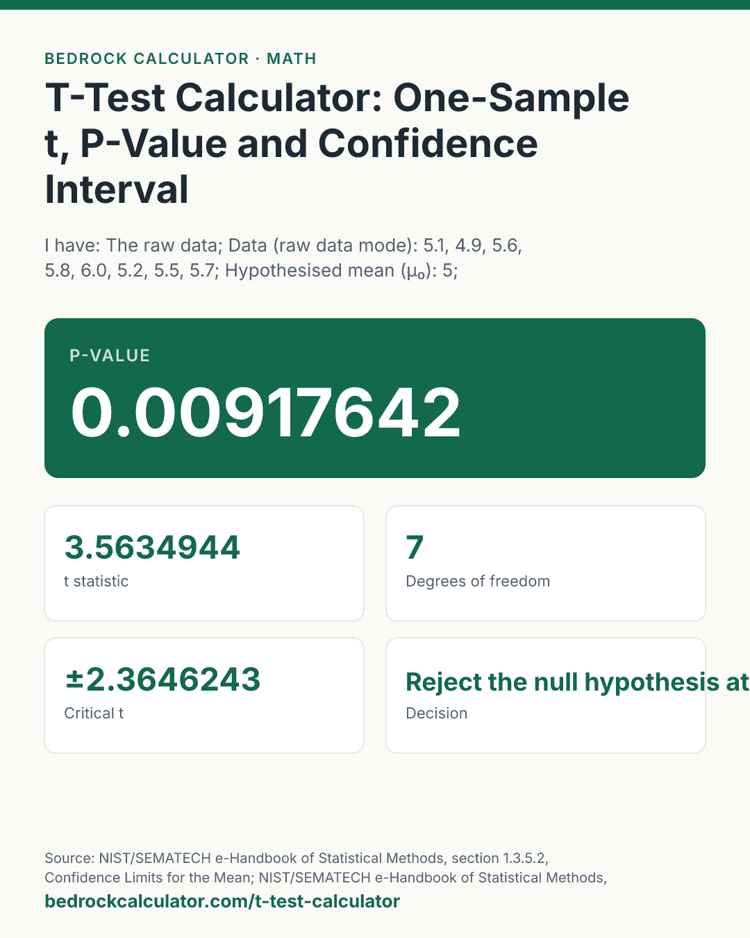

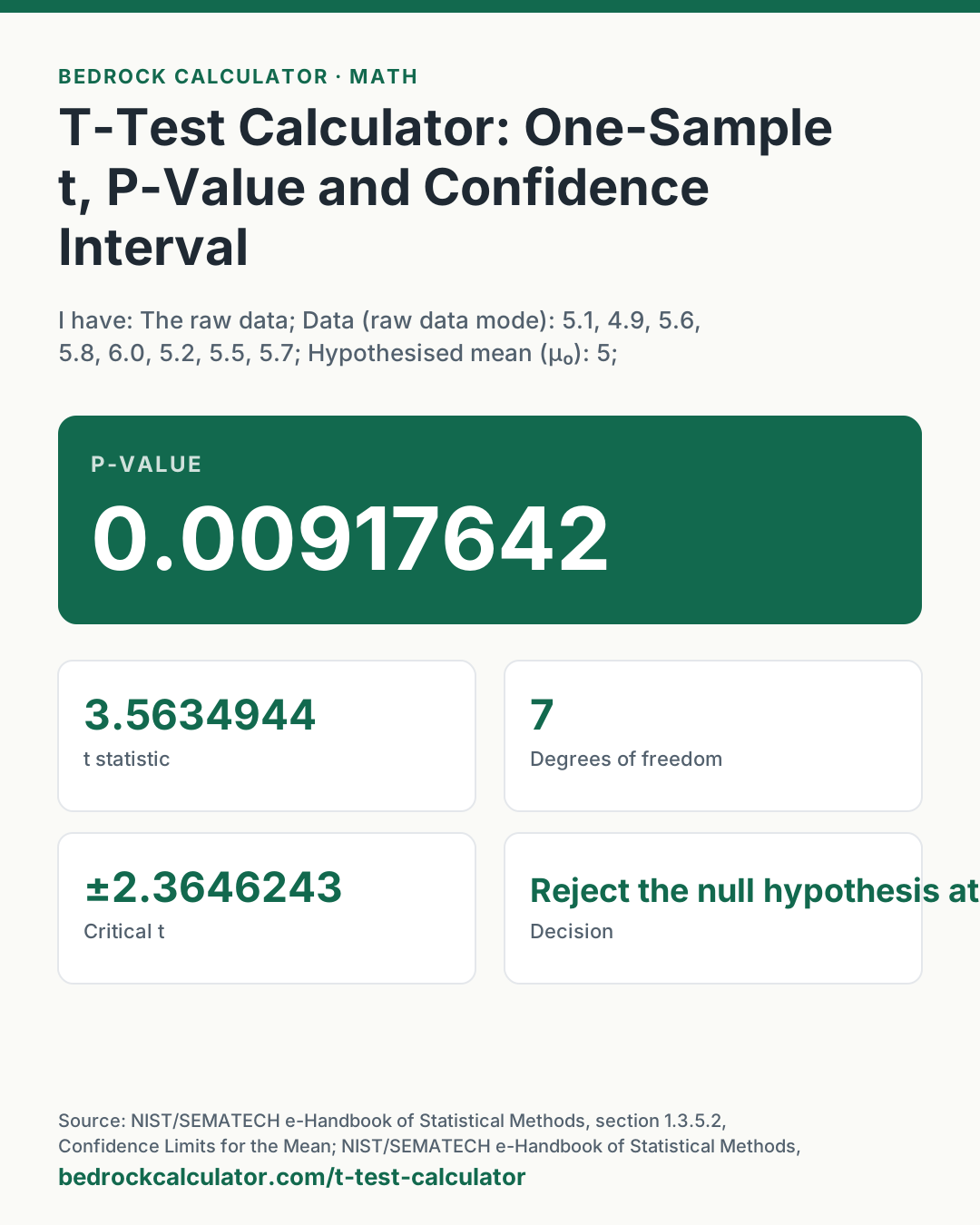
Quick Answer: For the data 5.1, 4.9, 5.6, 5.8, 6.0, 5.2, 5.5, 5.7 tested against a mean of 5, the two-tailed p-value is 0.0092: t is 3.563 with 7 degrees of freedom, and the 95% confidence interval for the mean runs from 5.160 to 5.790.
What does this calculator do?
This t-test calculator runs a one-sample t-test: it asks whether the mean of a sample is consistent with a hypothesised value, μ₀. It returns the t statistic, the degrees of freedom, the p-value for a two-tailed, right-tailed or left-tailed test, the critical t, a plain-language decision, and a confidence interval for the mean.
You can give it the raw data or just three summary numbers: the sample mean, the sample standard deviation and the sample size. Either way, the calculation follows the NIST/SEMATECH e-Handbook of Statistical Methods, which defines the test statistic, the n - 1 degrees of freedom and the confidence limits used here.
The t distribution is evaluated exactly for whole degrees of freedom, by a finite series rather than a numerical approximation, and the critical values agree with the NIST/SEMATECH table of the t distribution at every entry checked.
Using the T-Test Calculator
- Choose raw data or summary statistics.
- Enter the data, or the mean, standard deviation (the n - 1 version) and sample size.
- Enter the hypothesised mean μ₀, the value you are testing against.
- Pick the confidence level (90%, 95% or 99%) and the alternative hypothesis: two-tailed if any difference matters, right-tailed if you only care whether the mean is larger, left-tailed if only smaller.
- Read the p-value at the top and the decision below it. The interval card always shows a two-sided interval at the chosen confidence.
How is this calculated?
- Summarise the sample. In raw data mode, the mean and the sample standard deviation (dividing the sum of squared deviations by n - 1) are computed exactly from the list. In summary mode they are taken as entered.
- Standard error and t statistic. The standard error is the sample standard deviation divided by the square root of n. The t statistic is the distance from the sample mean to μ₀ in standard errors, with n - 1 degrees of freedom.
t = (x̄ − μ₀)/(s/√n); ν = n − 1
- Evaluate the t distribution. With θ = arctan(|t| / √ν), the probability that |T| is below |t| is a finite sum in powers of cos θ (Abramowitz and Stegun 26.7.3 for odd ν, 26.7.4 for even ν). For one degree of freedom it reduces to 2θ/π.
A(t|ν) = sin θ(1 + 1/2 cos ²θ + 1⋅3/2⋅4 cos ⁴θ + ⋯) (ν even)
- p-value. The upper tail is (1 - A)/2. A right-tailed p-value is the area above t, a left-tailed one the area below t, and a two-tailed one twice the area beyond |t|.
p_two = 1 − A(|t||ν)
- Critical t. With α equal to 1 minus the confidence level, the critical value is the t with an upper tail of α/2 for a two-tailed test and α for a one-tailed test. For 1 and 2 degrees of freedom it comes from the closed forms (tan(π(p - 1/2)) for one degree of freedom). Otherwise it starts from the Cornish-Fisher approximation and is refined by Newton's method on the exact distribution, using the t density with its gamma function ratio built exactly for whole ν, until the change is far below the digits shown.
- Confidence interval. The two-sided interval is the sample mean plus and minus the critical t for α/2 times the standard error, as in NIST/SEMATECH section 1.3.5.2. The margin of error card shows that half-width.
x̄ ± t_(1 − α/2, ν) s/√n
- Decision. If the p-value is below α, the null hypothesis is rejected at that level; otherwise it is not rejected. Values are shown with t to 8 significant figures and probabilities to 6, rounded half up.
Worked Example
The default data is eight measurements: 5.1, 4.9, 5.6, 5.8, 6.0, 5.2, 5.5, 5.7, tested against μ₀ = 5 at 95% confidence, two-tailed.
- Mean: 5.475. Sample standard deviation: 0.37701838.
- Standard error: 0.37701838 ÷ √8 = 0.13329613.
- t = (5.475 - 5) ÷ 0.13329613 = 3.5634944, with 7 degrees of freedom.
- Two-tailed p-value: 0.00917642. That is below 0.05, so the null hypothesis that the true mean is 5 is rejected at the 0.05 level.
- Critical t for 95%, two-tailed, 7 degrees of freedom: ±2.3646243. The t statistic is beyond it, which is the same conclusion.
- 95% confidence interval: 5.1598047 to 5.7901953. The interval does not contain 5.
The Mean 5.2, SD 0.4, n 16 preset is a summary-statistics example. The standard error is 0.1, so t = 2 with 15 degrees of freedom. The two-tailed p-value is 0.063945, not significant at 0.05, and the interval 4.986855 to 5.413145 contains 5. The Right-tailed version of the same numbers halves the p-value to 0.0319725, which is significant: a one-tailed test needs a smaller t to reach significance, which is why it should be chosen before looking at the data, not after.
How Do You Find Degrees of Freedom for a T-Test?
For a one-sample t-test, the degrees of freedom are the sample size minus one. A sample of 8 has 7; a sample of 16 has 15. One degree is used up because the deviations are measured from the sample's own mean, which forces them to add to zero, so only n - 1 of them are free to vary.
Two-sample and paired tests have their own rules, described below under what this calculator does not do.
Critical T-Values at 95% Confidence
The reference table lists the two-sided 95% critical values for common sample sizes. For 2 observations (1 degree of freedom) the critical value is 12.706205, for 11 (10 degrees of freedom) it is 2.2281389, and by 1,001 it has fallen to 1.9623391, close to the normal distribution's 1.96. These agree with the NIST/SEMATECH table, which prints 12.706, 2.228 and so on to three decimals.
What does this calculator not account for?
- Two samples. Comparing the means of two independent groups needs a two-sample t-test (pooled or Welch). That is not computed here.
- Paired data. For before-and-after measurements on the same subjects, subtract each pair and run this one-sample test on the differences against μ₀ = 0. That is exactly a paired t-test.
- Normality. The test assumes the data come from a roughly normal distribution, or that the sample is large enough for the mean to be close to normal. With small, strongly skewed samples the p-value can mislead. Nothing here checks the assumption.
- Known population standard deviation. If σ is known rather than estimated, the z-test applies; use the z-score calculator with the standard error as the standard deviation.
- Sample size limits. Sample sizes from 2 to 5,000 are accepted, which keeps the exact series fast enough to run as you type.
- Effect size and power. The p-value says nothing about how large or important a difference is, and no power analysis is done.
What mistakes do people make with this?
- Choosing the tail after seeing the data. Switching to a one-tailed test because the two-tailed p-value missed 0.05 doubles the real false-positive rate.
- Entering the population standard deviation. The test uses the sample standard deviation, s, with n - 1 in the divisor.
- Reading "do not reject" as "proved equal". A non-significant result means the data are consistent with μ₀, not that the mean equals μ₀.
- Treating the interval and the test as unrelated. A two-sided test at α rejects exactly when the (1 - α) interval excludes μ₀.
- Rounding the standard deviation too much. In summary mode, enter the standard deviation with as many digits as you have.
Frequently Asked Questions
What is a t-test used for?
What is the difference between a t-test and a z-test?
How do I get a confidence interval for a mean?
What does the p-value mean?
Is 0.05 the right significance level?
Sources
- NIST/SEMATECH e-Handbook of Statistical Methods, section 1.3.5.2, Confidence Limits for the Mean: the t statistic, degrees of freedom and interval. itl.nist.gov/div898/handbook/eda/section3/eda352.htm
- NIST/SEMATECH e-Handbook of Statistical Methods, section 1.3.6.7.2, Critical Values of the Student's t Distribution: the table the calculator is checked against. itl.nist.gov/div898/handbook/eda/section3/eda3672.htm
- NIST/SEMATECH e-Handbook of Statistical Methods, section 1.3.6.6.4, t Distribution: the density function. itl.nist.gov/div898/handbook/eda/section3/eda3664.htm
- NIST/SEMATECH e-Handbook of Statistical Methods, section 1.3.5.6, Measures of Scale: the sample standard deviation. itl.nist.gov/div898/handbook/eda/section3/eda356.htm