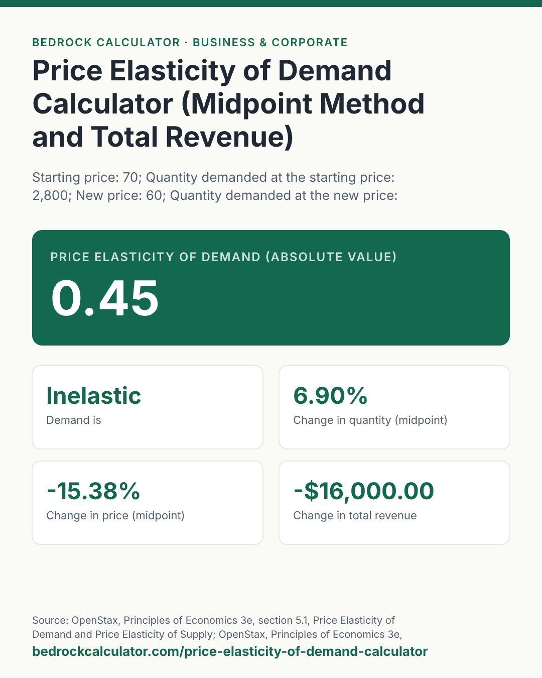

Quick Answer: When the price falls from $70 to $60 and sales rise from 2,800 to 3,000 units, the price elasticity of demand is 0.45: demand is inelastic, so the price cut lowers total revenue from $196,000 to $180,000.
What does this calculator do?
This price elasticity of demand calculator measures how strongly the quantity people buy responds to a change in price. Give it two points on a demand curve, a price and the quantity sold at it, before and after a change, and it returns the elasticity by the midpoint method, says whether demand is elastic or inelastic over that range, and works out total revenue at both points, the change in revenue and the marginal revenue over the move.
The defaults are the example used in OpenStax's Principles of Economics: a price cut from $70 to $60 that raises quantity demanded from 2,800 to 3,000. The book works it to an elasticity of 0.45, and so does the calculator.
Elasticity matters because it decides what a price change does to revenue. When demand is inelastic, a price rise brings in more money even though fewer units sell. When it is elastic, a price rise loses more in volume than it gains in price, and revenue falls. The calculator shows both the elasticity and the revenue change, so you can see the rule at work on your own numbers.
Using the Price Elasticity of Demand Calculator
- Enter the starting price and the quantity demanded at that price.
- Enter the new price and the quantity demanded at the new price.
- Read the elasticity at the top, as an absolute value, and whether demand is elastic, inelastic or unit elastic.
- Below it, check the percentage changes, total revenue before and after, the change in revenue, and marginal revenue.
The two prices must be different, and the quantities cannot both be zero. Quantities can be units per day, per week or per year, as long as both are measured over the same period. The presets load the book's second example ($120 to $130), a unit-elastic case, and a café raising the price of coffee.
How is this calculated?
- Percentage change in quantity, by the midpoint. The change in quantity is divided by the average of the two quantities, not by the starting one.
%ΔQ = (Q₂ − Q₁)/((Q₂ + Q₁)/2) × 100
- Percentage change in price, by the midpoint. The same with the two prices.
%ΔP = (P₂ − P₁)/((P₂ + P₁)/2) × 100
- Divide. The elasticity is the percentage change in quantity divided by the percentage change in price. Because price and quantity demanded usually move in opposite directions, the result is negative, and it is reported as its absolute value. The signed figure is shown too.
E_d = %ΔQ/%ΔP
- Classify. Above 1 is elastic, below 1 inelastic, exactly 1 unit elastic. If quantity does not change at all, demand is perfectly inelastic.
- Total revenue. At each point, total revenue is price times quantity.
TR = P × Q
- Marginal revenue. The change in total revenue divided by the change in quantity, over the move from one point to the other. It is undefined when the quantity does not change.
MR = (TR₂ − TR₁)/(Q₂ − Q₁)
- Simple method, for comparison. The calculator also divides each change by the starting value instead of the midpoint. That figure changes depending on which point you start from, which is why the midpoint method is the standard one.
- Round for display. Elasticities are shown to two decimal places (the simple one to three), percentages to two, and money to the cent.
Worked Example
With the default inputs, $70 to $60, and 2,800 to 3,000 units:
- Quantity change: 200 ÷ 2,900 × 100 = 6.9%.
- Price change: −10 ÷ 65 × 100 = −15.38%.
- Elasticity: 6.9 ÷ −15.38 = −0.45, reported as 0.45. Demand is inelastic.
- Total revenue before: $70 × 2,800 = $196,000.00. After: $60 × 3,000 = $180,000.00.
- Revenue change: −$16,000.00. The price cut lowered revenue, as inelastic demand predicts.
- Marginal revenue: −16,000 ÷ 200 = −$80.00 per extra unit sold.
Moving up the same curve, from $120 and 1,800 units to $130 and 1,600 units, gives an elasticity of 1.47: elastic. The price rise lowers total revenue from $216,000.00 to $208,000.00.
A café that raises coffee from $4.00 to $4.50 and sees daily sales fall from 500 to 470 cups faces an elasticity of 0.53. Demand is inelastic, and revenue rises from $2,000.00 to $2,115.00.
How Do You Calculate Total Revenue?
Multiply the price by the quantity sold: total revenue is P × Q. At $70 a unit and 2,800 units it is $196,000. Total revenue is the money that comes in before any costs, so it is not the same as profit.
Elasticity tells you which way total revenue moves when you change the price:
- Inelastic demand (below 1): raising the price raises total revenue; cutting it lowers revenue.
- Elastic demand (above 1): raising the price lowers total revenue; cutting it raises revenue.
- Unit elastic (exactly 1): revenue stays the same either way. The unit-elastic preset doubles the price from $10 to $20 and halves sales from 100 to 50, and revenue stays at $1,000.00.
The table below the calculator shows the switch-over. For a price cut from $100 to $90, revenue falls in every row up to 1,110 units, where the elasticity is still just under 1 at 0.99, and rises from 1,150 units, where it is 1.33.
What does this calculator not account for?
- Costs and profit. The calculator measures revenue, not profit. A price cut that raises revenue can still lower profit if each extra unit costs more to make than it brings in.
- Other things changing. Elasticity assumes only the price changed. If incomes, competitors' prices, seasons or advertising also changed between your two points, the quantity change mixes all of them.
- One stretch of the curve. The answer describes the range between your two prices. Demand can be inelastic at low prices and elastic at high ones, as the two OpenStax examples show.
- Long run versus short run. Buyers often adjust more over time. A short-run elasticity from one week's data can understate the long-run response.
- Upward-sloping demand. If quantity rises with price in your data, the signed elasticity is positive. The calculator reports it, but such data usually means something other than price changed.
What mistakes do people make with this?
- Dividing by the starting values only. The simple method gives a different answer depending on direction. For the default move it gives 0.5 rather than 0.45. Use the midpoint result to compare with textbooks and published estimates.
- Mixing time periods. Daily sales at one price and weekly sales at another produce a meaningless elasticity.
- Reading the sign as the size. An elasticity of −1.47 is more elastic than −0.45. Compare absolute values.
- Confusing elasticity with slope. A straight demand line has the same slope everywhere but a different elasticity at every point.
- Expecting revenue to follow quantity. Selling more units does not mean more revenue if the price had to fall a lot to get them.
Frequently Asked Questions
How do I calculate the price elasticity of demand?
What does an elasticity of 0.45 mean?
Is demand elastic or inelastic if the answer is above 1?
How do I compute total revenue from price and quantity?
What is marginal revenue?
Why use the midpoint formula?
Sources
- OpenStax, Principles of Economics 3e, section 5.1, Price Elasticity of Demand and Price Elasticity of Supply: the midpoint formula and the $70 to $60 and $120 to $130 examples. openstax.org/books/principles-economics-3e/pages/5-1-price-elasticity-of-demand-and-price-elasticity-of-supply
- OpenStax, Principles of Economics 3e, section 5.3, Elasticity and Pricing: total revenue as price times quantity and how elasticity decides its direction. openstax.org/books/principles-economics-3e/pages/5-3-elasticity-and-pricing
- OpenStax, Principles of Economics 3e, section 9.2, How a Profit-Maximizing Monopoly Chooses Output and Price: marginal revenue as the change in total revenue from selling more output. openstax.org/books/principles-economics-3e/pages/9-2-how-a-profit-maximizing-monopoly-chooses-output-and-price